Week 2 Air standard Cycle

Introduction

The air standard cycle is a thermodynamic power cycle that converts heat energy into mechanical power by considering air as a working fluid with constant specific heats (Cp & Cv).

In this cycle, the air is the only working fluid that goes through changes in its thermodynamic properties to convert heat into mechanical power.

Hence it works as a closed cycle with no mass transfer. Working fluid air is considered an ideal gas with constant specific heat.

The Air standard cycle assumptions are as follows:-

• Air is considered as working fluid.
• Air has constant specific heat.
• Air behaviour is ideal
• All processes in the cycle as internally reversible.
• For air Change in K.E.= 0, Change in P.E.= 0
• No internal heat generation.
• heat is added & rejected externally.
• The cycle is closed & processes are non-flow processes.
• There are no frictional losses.

Example for the Air standard cycle

• Carnot cycle
• Otto cycle or Petrol cycle
• Diesel cycle
• Air standard dual cycle
• Brayton cycle etc.

OTTO Cycle

Process 1-2:

Air is compressed isentropically to 13. Ratio V₁ to V₂ is called compression ratio donated by cr. Cover is adiabatic. At the end of compression.

Process 2-3:

At the end of compression, heat is added at constant volume by bringing a hot body near the cylinder diabatic cover. Heat is added at constant volume and hence pressure and temperature increase. Because the heat is added at a constant volume, the cycle is called as Constant Volume Cycle.

Process 3-4:

After heat is added, air expands isentropically to state 4. Here the expansion ratio is given by r_e = V₄/V₃. For Otto-cycle cr= ce. The adiabatic cover is kept during expansion.

Process 4-1:

At the end of the isentropic expansion. Heat is rejected at constant volume thus decreasing the pressure and temperature to initial values.

Thermal Analaysis

Heat supply = heat added during 2-3

`Q_s=m*c_v*(T3-T2)`

Heat rejection = heat rejection 4-1

`Q_R=m*c_v*(T4-T1)`

Work

`W=Q_s-Q_R`

Thermal Efficiency

`eta=(WORK DONE)/(HEAT SUPPLY)`

`eta=1-1/(cr^(gamma-1))`

or

`eta=(1-((t4-t1)/(t3-t2)))*100`

crank pin radius

`a = (stroke)/2`

constant

`R = (CONNECTING ROD)/(CRANK PIN RADIUS`

Volume Trace can be given for 1 to 2,3 to 4

number of points created in between = 30

theta in radian

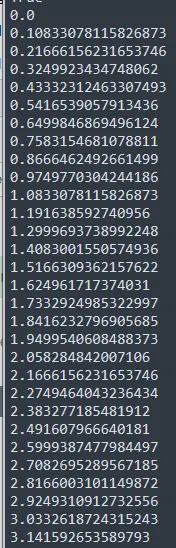
Volume Expansion from `theta=` 0 to 180 degree

Volume Compression from `theta=` 180 to 0 degree

`V=1+(1/2*(cr-1)+(R + 1 -costheta-(R^2-sintheta^2)^(1/2))*v_c`

Python Code

"""
ottocycle simulator
"""

import math
import matplotlib.pyplot as plt

def engine_kinematics(bore,stroke, con_rod, cr, start_crank, end_crank):

	a = stroke/2
	R = con_rod/a

	#stroke volume
	v_s = (math.pi/4)*pow(bore,2)*stroke
	#compression volume
	v_c = v_s/(cr-1)

	#volume trace
	#starting crank angle in radius
	sc = math.radians(start_crank)
	#ending crank angle in radius
	ec = math.radians(end_crank)

	#Number of inbetween state points
	num_values = 30

	#change in angle
	dtheta = (ec-sc)/(num_values- 1)

	# creating points for volume trace
	v=[]
	for i in range(0,num_values):
		theta = sc + i*dtheta
		
		
		term1 = 0.5*(cr-1)
		term2 = R + 1 - math.cos(theta)
		term3 = pow(R,2)- pow(math.sin(theta),2)
		term3 = pow(term3,0.5)
		v.append((1 + term1*(term2 - term3))*v_c)
	return v
	
# inputs
p1 = 101325
t1 = 500
gamma = 1.4
t3 = 2300

#Geometric parameters
bore = 0.1
stroke = 0.1
con_rod = 0.15
cr = 12

# volume computation
v_s = (math.pi/4)*pow(bore,2)*stroke

v_c = v_s/(cr-1)
v1 = v_c + v_s

#state point 2
v2 = v_c

#p2v2^gamma=p1v1^gamma
p2 = (p1*pow(v1,gamma))/(pow(v2,gamma))
print('validating pressure suction condition')
print('p2 > p1')
print(p2 > p1)

#p2v2/t2 = p1v1/t1 from rhs=p1v1/t1| rhs = p2v2/t2 | t2=p2v2/rho
rhs =  p1*v1/t1
t2 = p2*v2/rhs

v_compression = engine_kinematics(bore,stroke, con_rod, cr, 180,0)

constant = p1*pow(v1,gamma)
# P_compression*v_compression = constant
P_compression = []

for v in v_compression:
	P_compression.append(constant/pow(v,gamma))

# state point 1
v3 = v2

#p3v3/t3 = p2v2/t2 | rhs = p2v2/t2 | p3=rhs*t3/v3
rhs = p2*v2/t2
p3 = rhs*t3/v3

# check the states of combustion to validate the condition
print('validating pressure expansion condition')
print('p3 > p2')
print(p3 > p2)

v_expansion = engine_kinematics(bore,stroke, con_rod, cr, 0,180)

constant = p3*pow(v3,gamma)
# P_expansion*v_expansion = constant
P_expansion = []

for v in v_expansion:
	P_expansion.append(constant/pow(v,gamma))

#state point 4
v4 = v1

# p4v4*gmma =p3v3*gamma
p4 = p3*pow(v3,gamma)/pow(v4,gamma)
# p4v4/t4 = p3v3/t3
t4 = p4*v4/rhs

#thermal effiecency
eta= (1-(1/(pow(cr,(gamma-1)))))*100
print('thermal efficiency=',eta,'%')

#Plots

plt.plot([v2,v3],[p2,p3])
plt.plot(v_compression,P_compression)
plt.plot(v_expansion,P_expansion)
plt.plot([v4,v1],[p4,p1])
plt.grid()
plt.title('P vs V Diagram')
plt.xlabel('volume[m^3]')
plt.ylabel('Pressure [bar]')
plt.show()

Output

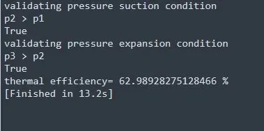
Graph

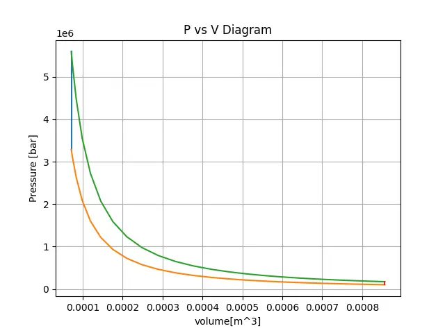
Conclusion

With Volume Trance we obtain the smooth output of the graph in an otto cycle

Thermal Efficiency =62.98%