Week 2 Air standard Cycle
AIM:
To write code that can solve an otto cycle and make plots for it using python.
OBJECTIVES:
- code should create a PV diagram
- the thermal efficiency of the engine.
OTTO CYCLE:
An Otto cycle is an idealized thermodynamic cycle that describes the functioning of a typical spark ignition piston engine. It is the thermodynamic cycle most commonly found in automobile engines.
The Otto cycle is a description of what happens to a mass of gas as it is subjected to changes of pressure, temperature, volume, addition of heat, and removal of heat. The mass of gas that is subjected to those changes is called the system. The system, in this case, is defined to be the fluid (gas) within the cylinder. By describing the changes that take place within the system, it will also describe in inverse, the system's effect on the environment. In the case of the Otto cycle, the effect will be to produce enough net work from the system so as to propel an automobile and its occupants in the environment.
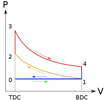
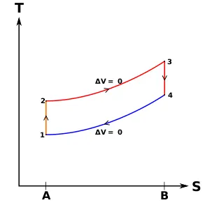
The Otto cycle is constructed from:
- Top and bottom of the loop: a pair of quasi-parallel and isentropic processes (frictionless, adiabatic reversible).
- Left and right sides of the loop: a pair of parallel isochoric processes (constant volume).
- The isentropic process of compression or expansion implies that there will be no inefficiency (loss of mechanical energy), and there be no transfer of heat into or out of the system during that process.
- The cylinder and piston are assumed to be impermeable to heat during that time. Work is performed on the system during the lower isentropic compression process. Heat flows into the Otto cycle through the left pressurizing process and some of it flows back out through the right depressurizing process.
- The summation of the work added to the system plus the heat added minus the heat removed yields the net mechanical work generated by the system.
PROCESS:
- Process 0–1 a mass of air is drawn into piston/cylinder arrangement at constant pressure.
- Process 1–2 is an adiabatic (isentropic) compression of the charge as the piston moves from bottom dead center (BDC) to top dead center (TDC).
- Process 2–3 is a constant-volume heat transfer to the working gas from an external source while the piston is at top dead center.
- This process is intended to represent the ignition of the fuel-air mixture and the subsequent rapid burning.
- Process 3–4 is an adiabatic (isentropic) expansion (power stroke).
- Process 4–1 completes the cycle by a constant-volume process in which heat is rejected from the air while the piston is at bottom dead center.
- Process 1–0 the mass of air is released to the atmosphere in a constant pressure process.
SOLUTION:
Now lets run a simulation of the Otto cycle using python.
PYTHON PROGRAM:
# Program to simulate the Otto cycle and plot the P-V diagram
# Engine Kinematics

# importing essential library tools
import math                     # importing math library
import matplotlib.pyplot as plt # importing ploting library
import numpy as np              # importing computing library
import scipy as sp              # importing scientific library

# Defining Engine Kinematics in a Function with bore, stroke, connecting rod, starting crank angle, ending crank angle
def EK(bore,stroke,conrod,Cr,startcrank,endcrank): # Creating a function for Engine kinematics

	# Engine Geometry
	a=stroke/2  # Crank pin radius
	r=conrod/a  # Ratio of crank radius to connecting rod

	# Volume parameters
	Vs=(math.pi/4)*pow(bore,2)*stroke  # Swept Volume
	Vc=Vs/(Cr-1)                       # Clearance Volume

	# Position of piston
	theta_startcrank=math.radians(startcrank)  # starting position of the crank
	theta_endcrank=math.radians(endcrank)      # ending position of the crank

	n=100                                           # Numerical value
	dtheta=(theta_endcrank-theta_startcrank)/(n-1)  # mean position of the crank
	v=[]                                            # user defined variable

	for i in range (0,n):                       # declaring a loop for simulation
		theta=theta_startcrank+i*dtheta         # expansion ratio to compression ratio
		term1=0.5*(Cr-1)                        # breaking the formula into 3 terms
		term2=r+1-math.cos(theta)               # ''''
		term3=(pow(r,2)-pow(math.sin(theta),2)) # ''''
		term3=pow(term3,0.5)                    # ''''
		v.append((1+term1*(term2-term3))*Vc)    # attaching the loop to the formula

	return v                                    # sending back the function to the loop

# Otto cycle Simulation

# Engine Parameters
bore=0.15   # Bore radius of cylinder
stroke=0.2  # stroke length
conrod=0.8  # connecting rod
Cr=10       # compression ratio

# input parameters
gamma=1.4  # ratio of specific heat
t3=2000    # temperature at state point 3

# state variables at point 1
p1=101324  # pressure at state point 1
t1=350     # pressure at state point 2

# Computing volume 1 and 2.
Vs=(math.pi/4)*pow(bore,2)*stroke  # swept volume
Vc=Vs/(Cr-1)                       # Clearance Volume
v1=Vs+Vc                           # Volume at state 1
v2=Vc                              # volume at state 2

# State variables at point 2
# isentropic compression
# p2*v2^gamma=p1*v1^gamma
p2=p1*pow(v1,gamma)/pow(v2,gamma)  # pressure at state 2

# p1*v1/t1=p2*v2/t2
t2=p2*v2*t1/(p1*v1)                # temperature at state 2

Vcomp=EK(bore,stroke,conrod,Cr,180,0)  # Compression of Volume
Cconst=p1*pow(v1,gamma)                # Constant volume
Pcomp=[]                               # Compression pressure

for v in Vcomp:                        # declaring Compression volume in loop
	Pcomp.append(Cconst/pow(v,gamma))  # attachind compression pressure along the loop

# State variables at point 3
v3=v2                                 # constant volume
# p3*v3/t3 = p2*v2/t2
p3=p2*v2*t3/(t2*v3)                   # Pressure at point 3

Vexp=EK(bore,stroke,conrod,Cr,0,180)  # Volume Expansion
Cconst=p3*pow(v3,gamma)               # constant
Pexp=[]                               # pressure Expansion

for v in Vexp:                        # declaring expansion volume in loop
	Pexp.append(Cconst/pow(v,gamma))  # attaching the pressure expansion along the loop

# State variables at point 4
v4=v1                              # Constant volume
# p3*v3^gamma = p4*v4^gamma
p4=p3*pow(v3,gamma)/pow(v4,gamma)  # pressure at point 4
# p3*v3/t3 = p4*v4/t4
t4=p4*v4*t3/(p3*v3)                # temperature in point 4

# plotting
plt.figure()  							# creating a figure
plt.plot(Vcomp,Pcomp)  					# ploting for istentropic compression
plt.plot([v2,v3],[p2,p3])  				# plotting for heat addition
plt.plot(Vexp,Pexp)        				# plotting for isentropic expansion
plt.plot([v4,v1],[p4,p1])  				# plotting for heat rejection
plt.xlim([0,0.005])        				# setting limits for x
plt.ylim([-5000,8000000])  				# setting limits for y
plt.xlabel('volume in m^3')  			# labeling the x axis
plt.ylabel('pressure in Pa')     		# labeling the y axis
plt.title('P-V diagram of Otto cycle')  # titling the plot

# Marking
plt.plot(v1,p1,'o')  # creating identification mark on plot
plt.text(v1,p1,'1')  # denoting it as 1
plt.plot(v2,p2,'o')  # creating identification mark on plot
plt.text(v2,p2,'2')  # denoting it as 2
plt.plot(v3,p3,'o')  # creating identification mark on plot
plt.text(v3,p3,'3')  # denoting it as 3
plt.plot(v4,p4,'o')  # creating identification mark on plot
plt.text(v4,p4,'4')  # denoting it as 4

# Display plot
plt.grid()  # turns on the grid lines on the figure
plt.show()  # displays the figure

# Computing Thermal Efficiency
TE=1-(1/pow(Cr,(gamma-1)))                                      # thermal Efficiency
print('thermal Efficiency of the otto cycle simulated is:',TE)  # Printing the thermal efficiency

# end
EXPLANATION:
- STEP 1 : Importing essential library tools.
initially we will be importing all the required libraries like math, plotting, numericals and scientific libraries. - STEP 2 : Defining the Engine Kinematics.
- The Engine kinematics as bore, stroke ,connecting road, start crank position and end crank position.
- we are using def command to define these factors in a function.
- the crank radius and ratio of crank radius to connecting road is defined in the Engine geometry.
- the volume parameters like swept volume and clearance volume is defined.
- the position of the crank i.e. start crank angle and end crank angle is defined. math.radians command is used to take the values in radians.
- the numerical values is defined as 100, the mean position of the crank is defined as dtheta followed by the expression.
- Now, we will be declaring a loop for simulation for that we are using for command and we assigning the loop to run from 0 to numerical value.
- using the expansion ratio to cutoff ratio we can find the combustion period.
- then, we will be splitting the expression into 3 terms.
- using append command we will be attaching the combustion period to the loop.
- with the help of return command we will be sending back the Engine kinematics functions to the loop of combustion.
- STEP 3 : OTTO CYCLE SIMULATION.
- initially we will be declaring the engine parameters like bore, storke, connecting road and compression ratio.
- then we will be declaring the input parameters like gamma and temperature of state point 3.
- now, will be declaring the state variables at point 1 like p1,t1 and for v1 it is the sum of swept volume and clearance volume.
- Since v2 is constant volume process v2 will be equal to the clearance volume and we will be declaring pressure at point2 and temperature at point 2.
- Now we will be calling the function under compression, that the piston will be in the BDC at 180, and we will be declaring compression in loop and attaching pressure along with pressure enabling heat addition.
- State 3 is isentropic expansion process, in this process we will doing the same derieving respected p,v values from expression.
- we will be again calling the function to perform the expansion process, where the piston moves to the TDC.
- Declaring expansion in loop and attaching pressure enabling heat rejection process.
- State 4, Constant volume het rejection, we will be getting v4,p4 and t4 from the respective ideal gas equation.
- STEP 4: PLOTTING.
- Now we will be plotting the PV diagram, for that we will using plt.figure() command and plt.plot to plot the required varibales.
- then with plt.xlim we will setting limits for the axe, followed by labelling and displaying.
- STEP 5: THERMAL EFFICIENCY.
- When we rewrite the expression for thermal efficiency using the compression ratio, we conclude the air-standard Otto cycle thermal efficiency is a function of compression ratio and κ = cp/cv.
- as per our simulation output, our system produces 0.60 i.e. 60 % of thermal efficiency.
OUTPUT:
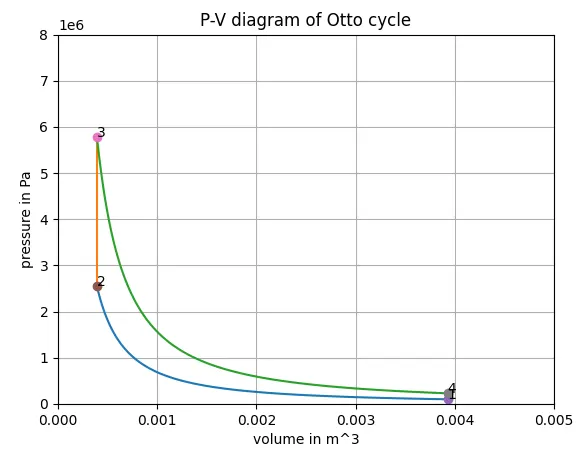
- The operation of the Otto cycle on a p-V diagram is shown in plot.
- The cycle comprises four processes:
- adiabatic compression 1 → 2,
- isochoric heat addition 2 → 3,
- adiabatic expansion 3 → 4,
- isochoric heat removal 4 → 1.
- Thus, for the Otto cycle, we have V2 = V3, V4 = V1, CR = V1/V3, and PR = p3/p1.
- The thermal efficiency of the Otto cycle is 60 %.

RESULT:
Thus the code that can solve an otto cycle is completed successfully using python and the output is verified.