Week 2 Air standard Cycle

Objective: To write a code that can solve an otto cycle and make plots for it. Also, calculate the thermal efficiency of the cycle.

Theory:

What is Otto Cycle?

The Otto Cycle describes how heat engines turn gasoline into motion. Like other thermodynamic cycles, this cycle turns chemical energy into thermal energy and then into motion. The Otto cycle describes how internal combustion engines (that use gasoline) work, like automobiles and lawnmowers.

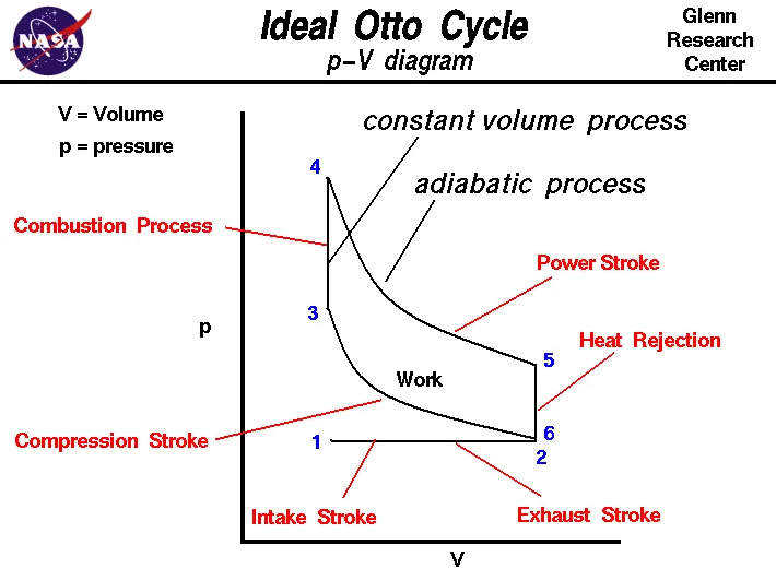
1-2: Referred to as the intake phase, the piston is drawn down to the bottom to allow the volume in the chamber to increase so it can "intake" a fuel-air mixture. In terms of thermodynamics, this is referred to as an isobaric process.

2-3: During this phase, the piston will be drawn up, so it can compress the fuel-air mixture that entered the chamber. The compression causes the mixture to increase slightly in pressure and temperature - however, no heat is exchanged. In terms of thermodynamics, this is referred to as an adiabatic process. When the cycle reaches point 3, that is when the fuel is met by the spark plug to be ignited.

3-4: This is where combustion occurs due to the ignition of fuel by the spark plug. The combustion of the gas is complete at point 4, which results in a highly pressurized chamber that has a lot of heat (thermal energy). In terms of thermodynamics, this is referred to as an isochoric process.

4-5: The thermal energy in the chamber as a result of combustion is used to do work on the piston - which pushes the piston down - increasing the volume of the chamber. This is also known as the power stroke because it is when the thermal energy is turned into motion to power the machine or vehicle.

5-6 and exhaust phase: From process 5 to 6, all waste heat is expelled from the engine chamber. As the heat leaves the gas, the molecules lose kinetic energy causing a decrease in pressure. Then the exhaust phase occurs when the remaining mixture in the chamber is compressed by the piston to be "exhausted" out, without changing the pressure.

Equation Required:

where,

V = Total volume

Vc = Clearnace volume

rc = Compression ratio

R = Radius of crank

`theta` = Crank angle

(Px * Vx) / Tx = (Py * Vy) / Ty

P * V^`gamma` = constant

Program Code:

Otto Cycle Simulator'
'Engine Kinematics'
'Created by Akhil'

import math
import matplotlib.pyplot as plt

def engine_kinematics (bore, stroke, con_rod, cr, start_crank, end_crank):
    
    # Geometric Parameters
    a = stroke/2
    R = con_rod/a
    
    # Volume Parameters
    v_s = math.pi * (1/4) * pow(bore, 2) * stroke   # Swept Volume
    v_c = v_s/(cr-1)                                # Clearance volume
    
    sc = math.radians(start_crank)   # Starting crank angle
    ec = math.radians(end_crank)     # Ending crank angle
    
    num_values = 40
    
    dtheta = (ec-sc)/(num_values-1)   # Crank angle spacing
    
    V = []
    
    for i in range(0, num_values):
        theta = sc + i * dtheta
    
        term1 = 0.5 * (cr-1)
        term2 = R + 1 - math.cos(theta)
        term3 = pow(R, 2)- pow(math.sin(theta), 2)
        term3 = pow(term3, 0.5)
    
        V.append((1 + term1 * (term2 - term3)) * v_c)
    
    return V
    
# Inputs
p1 = 101325
t1 = 500
gamma = 1.4
t3 = 2300
    
# Geometric Parameters
bore = 0.1
stroke = 0.1
con_rod = 0.15
cr = 7
    
# Volume computation
v_s = math.pi * (1/4) * pow(bore, 2) * stroke
v_c = v_s/(cr-1)
v1 = v_s + v_c
    
# State point 2
v2 = v_c

# P2 V2^gamma = P1 V1^gamma
p2 = p1 * (pow(v1, gamma) / pow(v2, gamma))

# P2 V2/T2 = P1 V1/T1 | RHS = P1 V1/T1 | P2 V2/T2 = RHS | T2 = P2 V2/RHS
rhs = (p1 * v1) / t1
t2 = (p2 * v2) / rhs

V_compression = engine_kinematics(bore, stroke, con_rod, cr, 180, 0)

constant = p1 * pow(v1, gamma)

P_compression = []

for v in V_compression:
    P_compression.append(constant/pow(v, gamma))


# State point 3
v3 = v2

# P3 V3/T3 = P2 V2/T2 | RHS = P2 V2/T2 | P3 V3/T3 = RHS | P3 = RHS * T3/V3
rhs = (p2 * v2) / t2
p3 = rhs * (t3 / v3)

V_expansion = engine_kinematics(bore, stroke, con_rod, cr, 0, 180)

constant = p3 * pow(v3, gamma)

P_expansion = []

for v in V_expansion:
    P_expansion.append(constant/pow(v, gamma))

# State point 4
v4 = v1

# P4 V4^gamma = P3 V3^gamma
p4 = (p3 * (pow(v3, gamma))/(pow(v4, gamma)))

# P4 V4/T4 = RHS
t4 = (p4 *v4)/rhs

plt.plot([v2, v3], [p2, p3])
plt.plot(V_compression, P_compression)
plt.plot(V_expansion, P_expansion)
plt.plot([v4, v1], [p4, p1])
plt.xlabel('Volume')
plt.ylabel('Pressure')
plt.savefig('Otto Cycle plot')
plt.show()

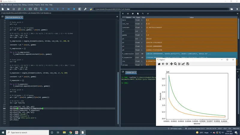
Program Window:

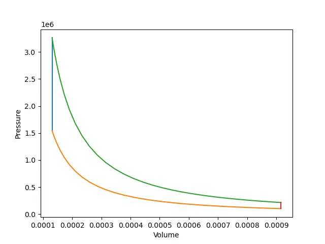
Graph:

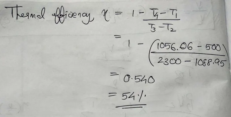
Thermal efficiency of this Otto Cycle:

Conclusion:

A code to plot the Otto cycle was written and compiled successfully. The thermal efficiency was also found out and came to be 54%.