Week 2 Air standard Cycle

1. Otto cycle (P-V) Diagram :

• The below code gives the PV diagram of a otto cycle.
• In writing the code the first approach was to note the values intail tempertatrure,pressure , value of gamma,bore diameter,stroke length,compression ratio (p1=1013251,t1=500,t3=2300,bore=0.1m,stroke=0.1m,con_rod=0.15,cr=12)
• Next step was to calculate swept volume and clearence volume using formula v_s=(math.pi/4)*pow(bore,2)*stroke and v_c=(v_s)/(cr-1).
• The intial volume v1 is calculated using v1=v_c+v_s and after isentropic compression v2 is given by v2=v_c.
• After isentropic compression p2 is given by p2=p1*pow(v1,gamma)/pow(v2,gamma)
• Since the compression stroke takes from 0 deg to 180deg and empty array for storing values of volumes corresponding to each angle is created and similarly pressure for corresponding volumes are calculated and stored in an array.
• Since the expansion stroke takes from 180 deg to 0deg and empty array for storing values of volumes corresponding to each angle is created and similarly pressure for corresponding volumes are calculated and stored in an array.
• Finaly graph is plotted for compression stroke , constant volume heat addtion and expansion stroke.

The below is the code for an otto cyle to obtain P-V diagram

import matplotlib.pyplot as plt
import math
def Engine(bore,stroke,con_rod,cr,start_crank,end_crank):
  a=stroke/2
  R=con_rod/a
  V_s=math.pi*(1/4)*pow(bore,2)*stroke
  V_c=V_s/(cr-1)

  sc=math.radians(start_crank)
  ec=math.radians(end_crank)
  
  num_values=50
  dtheta=(ec-sc)/(num_values-1)
  V=[]

  for i in range(0,num_values):
    theta=sc+i* dtheta
    term1=0.5*(cr-1)
    term2=R+1-math.cos(theta)
    term3=pow(R,2)-pow(math.sin(theta),2)
    term3=pow(term3,0.5)

    V.append((1+term1*(term2-term3))*v_c)
  return V  
  


gamma=1.4
p1=1013251
t1=500
t3=2300
# geometric parameter 
bore=0.1
stroke=0.1
con_rod=0.15
cr=12
#volume computation
#swept volume 
v_s=(math.pi/4)*pow(bore,2)*stroke
#clearence volume 
v_c=(v_s)/(cr-1)
v1=v_c+v_s
#state point 2
v2=v_c

p2=p1*pow(v1,gamma)/pow(v2,gamma)

rhs=(p1*v1)/t1
t2=(p2*v2)/rhs
V_comp=Engine(bore,stroke,con_rod,cr,180,0)
constant=(p1*pow(v1,gamma))
P_compression=[]
for v in V_comp:
  P_compression.append(constant/pow(v,gamma))


#state point 3
v3=v2

rhs=(p2*v2)/t2
p3=rhs*(t3/v3)
t3=(p3*v3)/rhs
V_exp=Engine(bore,stroke,con_rod,cr,0,180)
constant=(p3*pow(v3,gamma))
P_exp=[]
for v in V_exp:
  P_exp.append(constant/pow(v,gamma))

#state point 4
v4=v1
p4=p3*pow(v3,gamma)/pow(v4,gamma)
t4=(p4*v4)/rhs
plt.plot([v2,v3],[p2,p3])
plt.plot(V_comp,P_compression)
plt.plot(V_exp,P_exp)
plt.plot([v4,v1],[p4,p1])
plt.xlabel("Volume")
plt.ylabel("Pressure")
plt.title("P-V diagram of Otto cycle")
plt.show()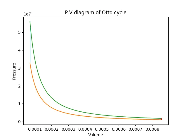

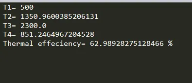
2) Calculating thermal effeciency of a otto cycle:

• For calculating thermal effeciency of a otto cycle

  Thermal effeciency=1-(t4-t1)/(t3-t2)

• The below shows the code :

• import matplotlib.pyplot as plt
  import math
  def Engine(bore,stroke,con_rod,cr,start_crank,end_crank):
    a=stroke/2
    R=con_rod/a
    V_s=math.pi*(1/4)*pow(bore,2)*stroke
    V_c=V_s/(cr-1)
  
    sc=math.radians(start_crank)
    ec=math.radians(end_crank)
    
    num_values=50
    dtheta=(ec-sc)/(num_values-1)
    V=[]
  
    for i in range(0,num_values):
      theta=sc+i* dtheta
      term1=0.5*(cr-1)
      term2=R+1-math.cos(theta)
      term3=pow(R,2)-pow(math.sin(theta),2)
      term3=pow(term3,0.5)
  
      V.append((1+term1*(term2-term3))*v_c)
    return V  
    
  
  
  gamma=1.4
  p1=1013251
  t1=500
  print("T1=",t1)
  t3=2300
  
  # geometric parameter 
  bore=0.1
  stroke=0.1
  con_rod=0.15
  cr=12
  #volume computation
  #swept volume 
  v_s=(math.pi/4)*pow(bore,2)*stroke
  #clearence volume 
  v_c=(v_s)/(cr-1)
  v1=v_c+v_s
  #state point 2
  v2=v_c
  
  p2=p1*pow(v1,gamma)/pow(v2,gamma)
  
  rhs=(p1*v1)/t1
  t2=(p2*v2)/rhs
  print("T2=",t2)
  V_comp=Engine(bore,stroke,con_rod,cr,180,0)
  constant=(p1*pow(v1,gamma))
  P_compression=[]
  for v in V_comp:
    P_compression.append(constant/pow(v,gamma))
  
  
  #state point 3
  v3=v2
  
  rhs=(p2*v2)/t2
  p3=rhs*(t3/v3)
  t3=(p3*v3)/rhs
  print("T3=",t3)
  V_exp=Engine(bore,stroke,con_rod,cr,0,180)
  constant=(p3*pow(v3,gamma))
  P_exp=[]
  for v in V_exp:
    P_exp.append(constant/pow(v,gamma))
  
  #state point 4
  v4=v1
  p4=p3*pow(v3,gamma)/pow(v4,gamma)
  t4=(p4*v4)/rhs
  print("T4=",t4)
  x=(t4-t1)/(t3-t2)
  TE=1-x
  TE=TE*100
  print("Thermal effeciency=",TE,"%")
  plt.plot([v2,v3],[p2,p3])
  plt.plot(V_comp,P_compression)
  plt.plot(V_exp,P_exp)
  plt.plot([v4,v1],[p4,p1])
  plt.xlabel("Volume")
  plt.ylabel("Pressure")
  plt.title("PV diagram of Otto cycle")
  plt.show()​

  
  Output:
• 
•