Air standard Cycle Using PYTHON

AIR STANDARD CYCLE USING PYTHON

PROBLEM STATEMENT-

The otto cycle is an idealized thermodynamic cycle which describes the spark ignition piston engine. Also known as the constant volume heat addition cycle, is highly used in automotive vehicles with petrol as fuel. To ease out calculations and study the change in graph for varying compression ratio, a software is used. Throughout this project, this cycle is solved using Python code to solve for :

• Pressure, volume and temperature at end points of ideal process
• Graphical representation of the otto cycle
• Calculation of thermal efficiency

GOVERNING EQUATIONS:

While coding, we assume the air as ideal gas. Various constant inputs in the equations are gamma(γ), compression ratio(cr),

Ideal gas equation PV /T = Constant (constant = mR; m - mass, R – universal Gas constant)

Isentropic Equation PV^γ =C ( γ = specific heat ratio= Cp/Cv)

Swept volume v_s = pi/4*bore^2*stroke

Clearance volume v_c = v_s/(cr-1)

Volume V= (1 + 0.5(cr- 1)((R + 1-cos(theta)) - ((R^2 - sin(theta)^2)^0.5))).*v_c

(R- engine rod ratio `theta`=crank angle cr- compression ratio)

Thermal efficiency E= 1- ((T4-T1)/(T3-T2))

INTRODUCTION-

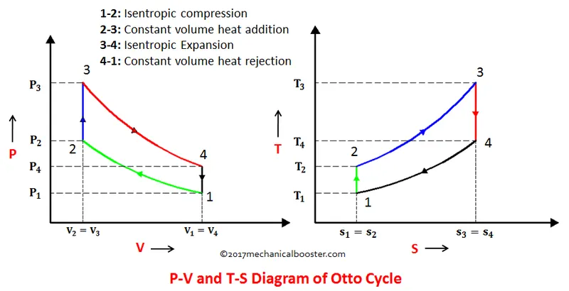
The Otto cycle is a thermodynamic cycle which consists of processes in spark ignition engine. It consists of following cycles:

1.Process 1–2 is an isentropic compression of the air, corresponding to the compression stroke. As the piston moves from the bottom to the top of the chamber, the internal energy, the temperature and the pression of the system increase, conserving the entropy.

2.Process 2–3 is a isochoric compression where heat is transferred into the air from an external source, resulting in a considerable increasing of the pressure. This process is intended to represent the ignition of the fuel–air mixture and the subsequent rapid burning.

3.Process 3–4 is an isentropic expansion corresponding to the power stroke, the air expands adiabatically, resulting in work into the system.

4.Process 4–1 isochoric decompression completes the cycle in which heat is rejected from the air while the piston is at the bottom, resulting in a decreasing of pressure. This process represents the exhaustion stroke where the valve opens to release the spent fuel-gas mixture.

Every factor of For the analysis, air-standard assumptions are made:

• Gas and air mixture are modelled as air and an ideal gas, which continuously circulates in a closed cycle. Thus, there are no intake and exhaust processes.
• All the processes making up the cycle are internally reversible.
• The combustion process is replaced by a heat-addition process from an external source.
• The exhaust process is replaced by a heat-rejection process and the gas returns to its initial state.

CODING –

For the code generation, python ide was used. First, let us have a brief about the whole procedure:

The libraries were imported to carry out calculation and plotting. Further, a function was created to obtain the Volume at various points of isentropic process. The input parameters and geometric parameters were provided. Using the basic formulae of thermodynamics, the pressure, temperature and volume was calculated for extreme points of various processes. Also, the pressure and volume was found for isentropic compression and expansion with the help of calling the previously developed function. At last, thermal efficiency was calculated by the formula and all the lines and points required were plotted.

#---------------------------------------------------#
#      OTTO CYCLE                                   |
#       Isentropic compression  (1 - 2)             |
#       Constant volume heat addition (2 - 3)       |
#       Isentropic expansion (3 - 4)                |
#       Constant volume heat rejection (4 - 1)      |
#---------------------------------------------------#

import math
import matplotlib.pyplot as plt


def engine_kinematics(bore,stroke,con_rod,cr,start_crank,end_crank): 
   
    #geometric parameters
    a = stroke/2
    R = con_rod/a
    
    #volume computation 
    vs = math.pi*(1/4)*pow(bore,2)*stroke    #swept volume
    vc = vs/(cr - 1)                         #clearance volume
    
    sc = math.radians(start_crank)           #starting crank angle
    ec = math.radians(end_crank)             #ending crank angle
    
    numvals = 50
    dtheta = (ec -sc)/(numvals-1)
    
    V = []                                   #void to store value
    for i in range(0,numvals):
        theta = sc + i*dtheta
        tm1 = (cr -1)*0.5
        tm2 = R + 1 - math.cos(theta)
        tm3 = pow((pow(R,2)- pow(math.sin(theta),2)),0.5)
    
        V.append((1 + tm1*(tm2 - tm3))*vc)   #append to capture next value
    return V                                 #return value to void
        

#inputs
p1 = 101325
t1 = 500
t3 = 2500
gamma = 1.4

#geometric parameters
bore = 0.1
stroke = 0.1
con_rod = 0.15
cr = 12                               #compression ratio

#volume computation
v_s = (math.pi/4)*pow(bore,2)*stroke   #swept volume
v_c = v_s/(cr - 1)                     #clearance volume        
v1 = v_s + v_c

#point 2 
v2 = v_c                              #BDC position
p2 = p1*pow(v1,gamma)/pow(v2,gamma)   #isentropic relation
t2 = 1/((p1*v1/t1)/(p2*v2))           #gas equation
V_comp = engine_kinematics(bore,stroke,con_rod,cr,180,0)

P_comp = []
for v in V_comp:
    P_comp.append((p1*pow(v1,gamma)/pow(v, gamma)))


#point 3
v3 = v2              
p3 = (p2/t2)*t3
V_exp = engine_kinematics(bore,stroke,con_rod,cr,180,360)

P_exp = []
for v in V_comp:
    P_exp.append((p3*pow(v3,gamma)/pow(v, gamma)))

#point 4
v4 = v1
p4 = p3*pow(v3,gamma)/pow(v4,gamma)
t4 = t1*(p4/p1)

#thermal efficiency
E = 1- ((t4-t1)/(t3-t2))

print(p1,v1,t1,"___",p2,v2,t2,"___",p3,v3,t3,"___",p4,v4,t4) 
plt.plot([v2,v3],[p2,p3],[v4,v1],[p4,p1])
plt.plot(V_comp,P_comp)
plt.plot(V_exp,P_exp)
plt.xlabel("Pressure")
plt.ylabel("Volume")
plt.show()

Let us discuss the working of function.

Using the command, a function was generated with variables bore, stroke, length of connecting rod, compression ratio, start crank angle and end crank angle. In this function our main objective is to calculate the volume for varies point in isentropic processes when the function is called for certain crank angle.

After writing the input parameters for engine rod ratio, clearance volume was calculated. This will further help to obtain volume swept at certain crank angle, as the code proceeds.

Math library will be used to change degrees to radian for starting crank angle(sc) and ending crank angle(ec). “numvals” and “dtheta” defines the interval for which calculation will be done. With increase in every interval, the value of theta(crank angle) will change. Hence as we increase the value of “numvals”, we will get smoother graph for volume points.

A void is created where volume will be stored as it returns. After this, a for loop is created to calculate volume at every point. In this for loop, range is given from zero to “numvals”, leading to calculation at every angle until the total reaches equal to “numvals”.

The theta is defined as progression in starting crank angle and with increase in value of dtheta according to increasing value of ‘i’. initial volume equation is broken into terms and then assembled together to form the volume output for particular crank angle.

The append command helps to add the previous result to the existing list. Hence we gave “.append” to volume. The return command in the end helps to return the value to void in which it is stored.

So, function has been created.

//---------------------------------------------------------------------------------------------------------------------------------------//

Now the calculation for various points are done using basic thermodynamics formulae. The provided parameters were Pressure and Temperature (1) at end of start of cycle and along with the temperature at the start of end of process 2. The further details consist of bore diameter, stroke length, connecting rod length, compression ratio (cr) and ‘γ’ (Cp/Cv). The aim was to calculate all the parameters in order to form PV diagram and find thermal efficiency of the cycle.

For calculation of volume at points 1 and 2, clearance and swept volume were calculated using the formulae given above. Hence p1 was calculated using isentropic relation.

From ideal gas equation, temperature t1 was calculated.

For point 3, temperature(t3) was given and volume(v3) was equal to the v2(isochoric heat addition) , pressure was calculated by ideal gas equation.

For point 4, volume was equal to that of point 1 (v4 = v1), pressure was calculated by isentropic equation and temperature was calculated using the ideal gas equation.

For the continuity of the isentropic processes, the function was called . Here calling for the function is done with input parameters as bore, stroke, connecting rod length, starting angle of crank and ending angle of crank. For isentropic compression, starting and ending crank angle was 180 and 0 respectively. For isentropic expansion, starting and ending crank angle was 180 and 360 respectively. Pressure was calculated using for loop and append command by the isentropic relations.

Thermal efficiency was calculated using temperatures rather than compression ratio in order to get the exact solution.

Further, matplotlib.pyplot library was used to get graphs and in the end plt.show() command was to display the graph in console.

RESULTS-

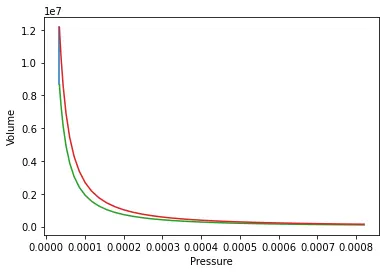
The results consists of formation of ideal graph for otto cycle. Further observation was done to understand the effect of compression ratio on thermal efficiency via this calculation

1. For compression ratio 8, thermal efficiency = 0.5647247183519378

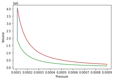
2. For compression ratio 10, thermal efficiency = 0.6018928294465026

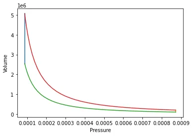
3. For compression ratio of 12, thermal efficiency = 0.6298928275128466

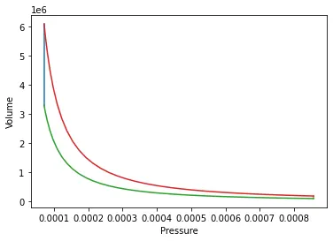
4. For compression ratio of 24, thermal efficiency = 0.7195112136384502 (this is just for calculation purpose. CR of this range is not used for Otto Cycle)

Observations –

• With increasing CR, the graph has increased pressure and volume difference after isentropic processes.
• The thermal efficiency increased with increase in compression ratio. This can be verified as validation of the code as in general thermal efficiency is a function of Compression Ratio by following formula :

Where r is the compression ratio

K is the specific heat ratio