Week 2 Air standard Cycle

Project Made By – Piyush Mishra

Aim

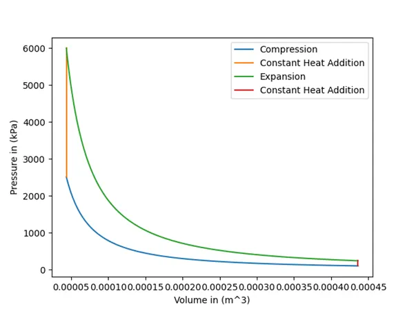
The main purpose of this project is to construct a Pressure vs Volume diagram for Otto Cycle and finding its efficiency via Python Coding

Governing Equations

There are few assumptions that need to be taken into account before constructing the PV diagram:-

1. Air is the only working fluid
2. Air is treated as perfect gas (not ideal gas)
3. But air follows Ideal Gas Equation
4. Specific heat capacity at a constant pressure of air (Cp = 1.005 kJ/kgK.) and Specific heat capacity at constant volume of air (Cv= 0.718 kJ/kgK.) both are constant
5. Internal combustion is modeled as a heat addition process that forms an External Source.
6. The exhaust process is modeled as a heat rejection process that restores the working fluid (air) at its initial state.

There are more than one equations of thermodynamics are used here:-

1. Ideal Gas Equation = PV = mRT

Where –P = Pressure (in kilo Pascal)

V = Volume (in m³)

m = mass of air (in kilogram)

R = Specific Gas Constant, equal to the Universal Gas Constant divided by the molar mass (M) of the gas or mixture. For air R = 0.287 kJ/kgK <We have directly used this number in programming>

2. Isentropic Equation è Pi Vi^γ = Pf Vf^γ è (Pi/Pf) = (Vf/Vi)^γ è (Pi/Pf) = (1/r)^γ

Where -- P_i = Initial Pressure (in kilo Pascal)

P_f = Final Pressure (in kilo Pascal)

V_i = Initial Volume (in m³)

V_f = Final Volume (in m³)

r = Compression Ratio <For otto cycle = 8-12>

γ = C_p/C_v = 1.4 <This is represented in code by “y”>

3. Efficiency of Otto Cycle è η = (1 – (1/r^(γ-1)))*100

Where -- η = Efficiency <This is represented in code by “E”>

r = Compression Ratio <Here, we use =10>

γ = C_p/C_v = 1.4 <This is represented in code by “y”>

γ = C_p/C_v = 1.4 <This is represented in code by “y”>

Geometry Explanation

Fact - The Stroke (height) of swept volume is equal Diameter of Crank (a) here. Hence

s = a/2 + (a/2 *Cos (θ))

Example è At θ = 0, Cos (θ) = 1 <BDC>

s = a/2 + a/2 = a

è At θ = π, Cos (θ) = -1 <TDC>

s = a/2 - a/2 = 0

Volume of Cylinder = Vc + Vs

= Vc + (π/4)*b²*s

= Vc + (π/4) * b² * [ a/2 + { a/2 * Cos (θ) } ]

<a=s is used so less variable is used>

Where-- Vc = Clearance Volume (in m³)

Vs = Swept Volume (in m³)

s = Stroke of Piston (in m)

b = Bore (Diameter) of Piston Head (in m)

θ = Angle between Crank Radius with horizontal axis

a = Diameter of Crank

Working of Internal Combustion Engine (Petrol Engine)

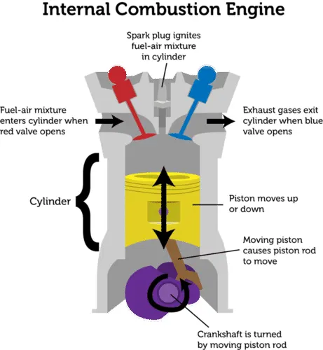
An internal combustion engine burns fuel internally, or inside the engine. This type of engine is found not only in cars but in most other motor vehicles as well. The engine works in a series of steps, which keep repeating.

1. A mixture of fuel and air is pulled-into a cylinder through a valve, which then closes.
2. A piston inside the cylinder moves upward, compressing the fuel-air mixture in the closed cylinder. The mixture is now under a lot of pressure and very warm.
3. A spark from a spark plug ignites the fuel-air mixture, causing it to burn explosively within the confined space of the closed cylinder.
4. The pressure of the hot gases from combustion pushes the piston downward.
5. The piston moves up again, pushing exhaust gases out of the cylinder through another valve.
6. The piston moves downward again, and the cycle repeats.

   Objectives of the Project

   Is to plot the variation of Pressure as crank angle changes. When crank angle changes the volume inside the cylinder also changes leading to different pressure values while going and returning from Bottom Dead Centre (0) to Top Dead Centre (π). So we can get a plot of Pressure-Volume Curve for Otto Cycle. And lastly calculate the efficiency of otto cycle.

   
   

   Body of Content

   Python Programing is used here with explanation:

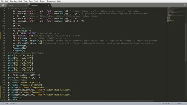
   import math
   import matplotlib.pyplot as pt
   import numpy as ny
   # Given Inputs
   P1 = 100 # in kPa <Initial Pressure is below always below the atmospheric Pressure>
   T1 = 300 # in K
   T3 = 1800 # in K
   r = 10 # Compression Ratio of petrol = V1/V2
   y = 1.4 # Value of gamma in air
   b = 0.05 # Dia of cyclender in m
   s = 0.2 # Stroke of cylinder in m
   Pc = [] # Defining an Null Array for Compression Pressure
   Pe = [] # Defining an Null Array for Expansion Pressure
   V = [] # Defining an Array for Volume <It's main use is while ploting as both x and y plots need to of same dimensions>
   for t in ny.linspace(0,math.pi,180): # t here means angle Theta <We are creating an array for value for theta in for loop as for every value theta swept volume changes>
   # Volume Calculation 	
   	Vs = math.pi/4*b*b * (  s/2 + (s/2 * math.cos(t))  ) # Swept Volume in m^3 at different position of crank radius
   	Vc = math.pi/4*b*b * (  s/2 + (s/2 * math.cos(0))  ) / (r-1) # Clearance Volume in m^3 <here swept volume should be max>
   	v = Vc + Vs # Volume of different positions of theta as swept volume changes
   	V1 = math.pi/4*b*b * (  s/2 + (s/2 * math.cos(0))  ) + Vc
   	V2 = math.pi/4*b*b * (  s/2 + (s/2 * math.cos(math.pi))  ) + Vc 
   	V3 = V2
   	V4 = V1
   # Pressure Calculation 	
   	P2 = P1*pow(r,y)
   	m = P1*V1/(0.287*300) # mass of air in kg
   	P3 = m*0.287*T3/V3 # 0.287 kJ/kgK is the value of R in PV=mRT 
   	P4 = P3/pow(r,y)	# (V3/V4) = (V2/V1) = (1/r)
   	pc = P1*pow(V1,y)/pow(v,y) # Compression Pressure of different positions of theta as swept volume changes in Compression process
   	pe = P3*pow(V3,y)/pow(v,y) # Expansion Pressure of different positions of theta as swept volume changes in Expansion process
   	Pc.append(pc)
   	Pe.append(pe)
   	V.append(v)
   # Printing Some Important Values
   print('V1 =',V1,'m^3')
   print('V2 =',V2,'m^3')
   print('Mass =',m,'kg')
   print('P1 =',P1,'kPa')
   print('P2 =',P2,'kPa')
   print('P3 =',P3,'kPa')
   print('P4 =',P4,'kPa')
   # Efficiency Calculation
   E = (1-(1/pow(r,(y-1))))*100
   print('Efficiency = ',E,'%')
   # Plotting Values
   pt.xlabel('Volume in (m^3)')
   pt.ylabel('Pressure in (kPa)')
   pt.plot(V,Pc, label="Compression")
   pt.plot([V2,V3],[P2,P3], label="Constant Heat Addition")
   pt.plot(V,Pe, label="Expansion")
   pt.plot([V1,V4],[P1,P4], label="Constant Heat Addition")
   pt.legend()
   pt.show()​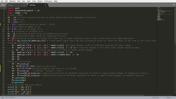

   

   

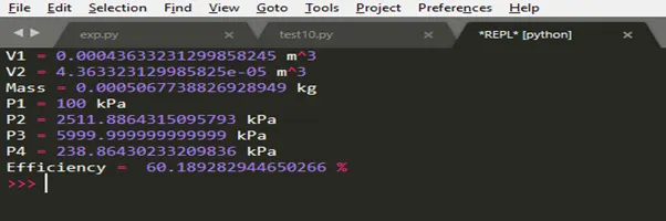
   It’s Output

   

   The Graph

   

   Conclusion

   We have plotted PV diagram and found out the efficiency for the same as well.