Week 2 Air standard Cycle

Problem Statement:

Write a program in MATLAB to plot the PV diagram and find the thermal efficiency of an engine running on the otto/air standard cycle.

Theory:

Otto Cycle -

In 1876, a German engineer, Nikolaus August Otto advanced the study of heat engines by building the first working four-stroke engine. The cycle of the Otto engine is called the Otto cycle. It is the one of most common thermodynamic cycles that can be found in automobile engines and describes the functioning of a typical spark ignition piston engine. In an ideal Otto cycle, the system executing the cycle undergoes a series of four internally reversible processes: two isentropic (reversible adiabatic) processes alternated with two isochoric processes.

PV Diagram -

A pressure-volume diagram is used to describe the corresponding changes in the volume and pressure of a system. The PV diagram can be used to find the work done as it is equal to the area enclosed under the PV diagram. For an otto cycle, the ideal and actual PV diagrams are as follows -

The processes involved in an ideal otto cycle are -

1->2 (Isentropic Compression) - The gas (fuel-air mixture) is compressed adiabatically from state 1 to state 2, as the piston moves from bottom dead center to top dead center. The surroundings do work on the gas, increasing its internal energy (temperature) and compressing it. On the other hand, the entropy remains unchanged.

2->3 (Isochoric Compression) - In this phase, there is a constant-volume (the piston is at rest ) heat transfer to the air from an external source while the piston is at rest at the top dead center. This process is intended to represent the ignition of the fuel–air mixture injected into the chamber and the subsequent rapid burning. The pressure rises and the ratio (P₃ / P₂) is known as the “explosion ratio”.

3->4 (Isentropic Expansion) - The gas expands adiabatically, as the piston moves from top dead center to bottom dead center. The gas does work on the surroundings (piston) and loses an amount of internal energy equal to the work that leaves the system. Again the entropy remains unchanged.

4->1 (Isochoric Expansion) - In this phase, the cycle completes by a constant-volume process in which heat is rejected from the air while the piston is at the bottom dead center. The working gas pressure drops instantaneously.

Isentropic Process - it is a thermodynamic process, in which the entropy of the fluid or gas remains constant.

Isochoric Process - It is a thermodynamic process, in which the volume of the closed system remains constant (V = const). It describes the behavior of gas inside the container, that cannot be deformed.

Thermal efficiency -

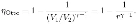
For a thermodynamic cycle, it is the ratio of the work output for a given amount of heat input. For the otto cycle, it can be derived as follows -

- IT IS THE HEAT ABSORBED

QL - IT IS THE HEAT LOST TO SURROUNDINGS

U - IT IS THE CHANGE IN INTERNAL ENERGY

Cv - IT IS THE MOLAR SPECIFIC HEAT AT CONSTANT VOLUME OF A GAS

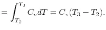Substituting the expressions for the heat absorbed and rejected in the expression for thermal efficiency yields -

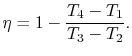
We can simplify the above expression using the fact that the processes from 1 to 2 and from 3 to 4 are isentropic:

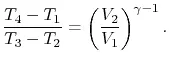
The quantity is called the compression ratio. In terms of compression ratio, the efficiency of an ideal Otto cycle is:

About the program:

# Engine Kinematics 
import math # import math library
import matplotlib.pyplot as plt # import plotting library

#defining a function to generate the values of volumeas per crank angle
def engine_kinematics(bore, stroke, con_rod, CR, start_crank, end_crank):

	a= stroke/2 # crank pin radius
	R = con_rod/a

	Vs =(math.pi/4)*pow(bore,2)*stroke #swept volume
	Vc = Vs/(CR - 1) #clearance volume

	sc = math.radians(start_crank) 
	ec = math.radians(end_crank)

	num_values = 30

	d_theta = (ec-sc)/(num_values - 1) 
	V = [] #null matrix for volume
	# for each value of theta, we find the volume using the engine kinematics formula
	for i in range(0,num_values):
		theta = sc + i*d_theta
		term1 = 0.5*(CR - 1) # the formula has been divided into terms to simplify it
		term2 = R + 1 - math.cos(theta)
		term3 = pow(R,2) - pow(math.sin(theta),2)
		term3 = pow(term3,0.5)
		V.append(Vc*(1 + term1*(term2-term3)))
	return(V) #since we want the compiler to return the value after the calculations

#intial conditions 
p1 = 101325
t1 = 500
t3 = 2300
gamma = 1.4

#geometric parameters
bore = 0.1
stroke = 0.1
con_rod = 0.15
CR = 12

#volume computation 
Vs =(math.pi/4)*pow(bore,2)*stroke
Vc = Vs/(CR - 1)
V1 = Vc + Vs

#Values at point 2 after isentropic compression
V2 = Vc 
p2 = p1*pow(V1,gamma)/pow(V2,gamma) #p1v1^gamma = p2v2^gamma 
rhs= p1*V1/t1
t2 = p2*V2/rhs

# we call the formula to get the values of volume for isentropic compression 
#where the movement is non linear adn so is the compression 
V_compression = engine_kinematics(bore, stroke, con_rod, CR, 180, 0)
constant = p1*pow(V1,gamma)

P_compression = []
for v in V_compression:
	P_compression.append(constant/pow(v,gamma))

#Values at point 3 after constant volume combustion
V3 = V2 
rhs = p2*V2/t2
p3 = rhs*(t3/V3)

#Values at point 4 after isentropic expansion
V4 = V1
p4= p3*pow(V3,gamma)/pow(V4,gamma) # p3v3^gamma = p4v4^gamma
rhs = p3*V3/t3
t4 = p4*V4/rhs

# we call the formula to get the values of volume for isentropic expansion
#where the movement is non linear adn so is the expansion 
V_expansion = engine_kinematics(bore, stroke, con_rod, CR, 0, 180)
constant = p3*pow(V3,gamma)

P_expansion = []
for v in V_expansion:
	P_expansion.append(constant/pow(v,gamma))

#Thermal Efficiency

Eta_T = (1 - (1/(pow(CR,(gamma-1)))))*100
print('The value of thermal efficiency is',Eta_T)

plt.plot([V2,V3],[p2,p3])
plt.plot([V4,V1],[p4,p1])
plt.plot(V_compression,P_compression)
plt.plot(V_expansion,P_expansion)
plt.show()

-> The program starts with defining a function that outputs the volume as per the given crank angles using a relation of engine kinematics given as -

-> This is followed by providing some basic dimensions of the engine and some initial conditions. Using these and the equations of gas law and isentropic volume change, we derive the values of the various points after each process. The volume after the isentropic compression and isentropic expansion is derived using the function we defined at the start of the program.

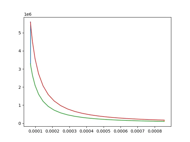
-> Lastly, we calculate and display the value of thermal efficiency and plot the values of pressures and volumes to obtain the PV diagram.

Output -