Week 2 Air standard Cycle

Week 2 Challenge - Air Standard Cycle

Objective:

To plot the PV diagram of an engine operating under the Otto cycle and to calculate the thermal efficiency of the engine.

Problem Statement:

To plot the PV diagram of an Otto cycle, we need to calculate the pressures, volumes and temperatures of each stage of the cycle. During the isentropic compression and isentropic expansion stages, the change in pressure and volume is not linear as in the constant volume heat addition and heat rejection stages.

In the isentropic compression and expansion stages, we need to determine the volume trace of the engine to accurately plot the PV diagram. Using the determined temperature values at each stage, need to find the thermal efficiency of the engine.

Solution:

To calculate the pressures, volumes, and temperatures at all four stages of the Otto cycle, we need to use the existing thermodynamic relations between all 3 parameters. We also need to assume starting state parameters and geometric parameters such as starting temperature, bore, stroke etc.

To plot the isentropic compression and expansion stages of the PV diagram, we can use a function that calculates the volume of the engine at a given value of the crank angle. Once the volume is known, we can use thermodynamic relations to calculate the respective pressure. This is done for compression and expansion stages.

To calculate the thermal efficiency, we can use a data book and determine the specific internal energy values of standard air at the temperature values. From the specific internal energy, we can derive the thermal efficiency.

Procedure:

First, open a new Python script and import the "math" and "matplotlib" libraries. Next, the assumed values of the state inputs are entered. The initial pressure "p1" is defined as 101325 Pascals which is equal to 1 bar. The initial temperature "t1" is defined as 500K. The temperature at state point 3, "t3" is defined as 2300K. The constant gamma is defined as 1.4.

Then, the geometric parameters of the engine are specified. The bore is defined as 0.1m. The stroke and connecting rod lengths are defined as 0.2m. The compression ratio "cr" is defined as 12 which is in the normal range of engines operating under the Otto cycle.

This is shown in the section below:

import math
import matplotlib.pyplot as plt 

# State Inputs
p1 = 101325
t1 = 500
t3 = 2300
gamma = 1.4

# Geometric Parameters
bore = 0.1
stroke = 0.2
con_rod = 0.2
cr = 12

In the next section, a function called "engine_kinematics" is created to calculate the volume trace of the engine during the isentropic compression and expansion stages. This function requires the inputs of bore, stroke, connecting rod length, compression ratio and start and end crank angles.

This function uses relation between volume and crank angle to perform this calculation. This relation is shown below:

`V/V_c = 1 + 0.5(cr-1)[R + 1 - costheta-(R^2-sin(theta)^2)^0.5]`

Where,

V - Swept Volume

`V_c` - Clearance Volume

`theta` - Crank Angle `

R - `(con__rod) / (a)`

a - `(stroke) / 2`

Next, the stroke volume and clearance volumes are calculated using the following formulae:

`v_s = pi/4 * D^2 * L`

`v_c = v_s / (cr -1)`

Where,

`v_s` - Swept Volume

D - Bore

L - Stroke Length

`v_c` - Clearance Volume

cr - Compression Ratio

This is shown in the section of code below:

def engine_kinematics(bore, stroke, con_rod, cr, start_crank, end_crank):

	a = stroke/2
	R = con_rod/a

	# Volume Trace
	# V/Vc = 1 + 0.5(cr-1)[R+1-costheta-(R^2-sin(theta)^2)^0.5]

	# Stroke Volume
	v_s = (math.pi/4) * pow(bore, 2) * stroke

	# Clearance Volume
	v_c = v_s/(cr-1)

Since the function requires the input arguments of start crank and end crank angles, we need to define them. Variables "sc" and "ec" are created which convert the value of the angle entered in the function arguments to radians.

A variable "num_values" is created and defined to 30. This variable is to be used in the upcoming for loop to generate an array of angle values for the volume trace. Another variable "dtheta" is created which calculates equal intervals between the start and end crank angles for the for loop.

An empty array for the volumes is created to store the volume values. A for loop is started which loops for the same number of times as defined by "num_values". The for loop will calculate equally spaced theta values which will be used in the volume trace calculation.

For simplicity, the volume trace equation is broken in to three terms or variables. Terms 2 and will include the value of theta in their calculation. Once all three terms are calculated, the volume value from each loop will be added to the empty array using the "append" command.

This is shown in the section of code below:

	
	sc = math.radians(start_crank)
	ec = math.radians(end_crank)

	num_values = 30
	dtheta = (ec-sc)/(num_values - 1)

	v = []

	for i in range(0, num_values):
		theta = sc + i*dtheta

	
		term1 = 0.5*(cr-1)
		term2 = R + 1 - math.cos(theta)
		term3 = pow(R, 2) - pow(math.sin(theta), 2)
		term3 = pow(term3, 0.5)

		v.append(v_c*(1 + term1*(term2 -term3)))
		
	return(v)

Then, the stroke and clearance volumes are defined once more for the upcoming calculations of the volume, temperature, and pressure for the remaining state points. In addition, the volume during state point 1 is equal to the sum of the swept and clearance volumes. This volume is defined as "v1".

For state point 2, the volume is the same as the clearance volume. So "v2" is defined as being equal to "v_c". To find the pressure at this state point, the following equation is used:

`p_2*v_2^gamma = p_1*v_1^gamma`

Since all the terms in the equation are known, we can solve for "p2". As this is a compression stage, the value of "p2" must be greater than "p1". The "print" command is used to confirm this.

To find the temperature at this state point, "t2", the ideal gas law is used. This is shown in the equation below:

`(p_2*v_2)/t_2 = (p_1*v_1)/t_1`

Since all the terms in the equation are known, we can solve for the unknown value of "t2". As this is a compression stage, the temperature value of "t2" will also be greater than "t1". The "print" command is used to confirm this.

Next, the "engine_kinematics" function is called to perform the volume trace calculations for the isentropic compression stage. During this stage, the piston travels from the Bottom Dead Center (BDC) to the Top Dead Center (TDC). During this transition, the crank angle varies from 180 degrees to 0 degrees. The start crank and end crank angles are entered as input arguments in to the function. The value of this calculation is equated to the variable "v_comp".

Next, the corresponding pressure value is also required for the respective "v_comp" values. In order to find this, we must use an existing relation that is shown below:

`p_1*v_1^gamma = c`

In this relation, c is a constant. By finding the value of the constant, we can work backwards and find the compression pressure values from the compression volume values. Since we have more than one value for the pressure, I will store them in an array.

An empty array for the compression pressures values is created first. Then, a for loop is created to perform the calculation and will loop for the same number of values in the compression volume array. For every loop, the values are added to the empty array using the "append" command. This is shown in the section of code below:

# Stroke Volume
v_s = (math.pi/4) * pow(bore, 2) * stroke

# Clearance Volume
v_c = v_s/(cr-1)
v1 = v_s + v_c
print(v1)

# STATE POINT 2 (ISENTROPIC COMPRESSION)

v2 = v_c

# To find p2 : p2v2^gamma = p1v1^gamma

p2 = (p1*pow(v1, gamma)) / (pow(v2, gamma))
print (p2)

# To find t2: p2v2/t2 = p1v1/t1

t2 = (p2*v2*t1)/(p1*v1)
print(t2)

v_comp = engine_kinematics(bore, stroke, con_rod, cr, 180, 0)
constant = p1*pow(v1, gamma)
p_comp = []
for v in v_comp:
	p_comp.append(constant/pow(v, gamma))

For state point 3 i.e. constant volume heat addition, the value of "v3" is defined as equal to "v2". This is because the volume does not change during this stage. As done previously, the value of the pressure at this stage is determined using the known values. This is shown in the section below:

# STATE POINT 3 (CONSTANT VOLUME HEAT ADDN.)

v3 = v2

# To find p3: p3v3/t3 = p2v2/t2
p3 = (p2*v2*t3)/(t2*v3)
print(p3)

For state point 4 i.e. isentropic expansion, since this is a closed system, we assume that the volume at this stage will be equal to the initial volume "v1". As such, this relation is defined in the variable "v4". To find the pressure at this point, "p4", we use existing thermodynamic relations as done previously.

Using the ideal gas equation, the temperature at this point, "t4", is determined as done for the isentropic compression stage.

Then, the "engine_kinematics" function is called to calculate the volume trace during this stage. During this stage, the piston travels from the TDC to the BDC and the crank angle varies from 0 to 180 degrees. The start and end crank angles are entered in to the function as the input arguments for this stage.

The values of the expasion volume are equated to the variable "v_expans". Then, the value of the expansion pressure is also calculated using the value of the constant during this stage as done previously for isentropic compression. An empty array for expansion pressure, "p_expans" is created. A for loop is used to calculate the value of expansion pressure. The values are added to the empty array using the "append" command.

This is shown in the section of code below:

# STATE POINT 4 (ISENTROPIC EXPANSION)

v4 = v1

# To find p4: p4v4^gamma = p3v3^gamma

p4 = p3*pow(v3, gamma)/pow(v4, gamma)
print(p4)

# To find t4 : p4v4/t4 = p3v3/t3

t4 = (p4*v4*t3)/(p3*v3)
print(t4)

v_expans = engine_kinematics(bore, stroke, con_rod, cr, 0, 180)
constant = p3*pow(v3, gamma)
p_expans = []

for v in v_expans:
	p_expans.append(constant/pow(v, gamma))

To calculate the thermal efficiency of the engine during the Otto cycle, we need to use the equation given below:

`eta = 1 - [(u_4 - u_1)/(u_3 - u_2)]`

Where,

`eta`- Thermal Efficiency of Engine

`u_1` - Specific Internal Energy of Engine at "t1" in kJ/kg

`u_2` - Specific Internal Energy of Engine at "t2" in kJ/kg

`u_3` - Specific Internal Energy of Engine at "t3" in kJ/kg

`u_4` - Specific Internal Energy of Engine at "t4" in kJ/kg

The values of the specific internal energy can be found in a data book containing the thermodynamic properties of air at 101325 Pa at the respective temperatures. For my temperature values, the specific internal energies were determined and used to calculate the thermal efficiency. This is shown in the section of code below:

# Thermal Efficiency (eta) calculation
u1 = 359.8
u2 = 1068
u3 = 1970
u4 = 633.5

eta = 1 -(u4-u1)/(u3-u2)
print(eta)

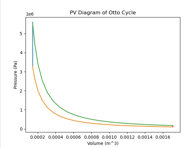
Finally, the PV diagram is plotted using the "plt.plot" command. This command is used four times. The first time, it is used to plot the volumes and pressures at state points 2 and 3. The second time, it is used to plot the compression volumes and pressures. The third time, it is used to plot the expansion volumes and pressures. The fourth time, it is used to plot the pressure and volume values at state points 4 and 1.

The plot is added with axes labels and a title for better representation and readability. This is shown in the section of code below:

# Plotting

plt.plot([v2, v3], [p2, p3])
plt.plot(v_comp, p_comp)
plt.plot(v_expans, p_expans)
plt.plot([v4, v1], [p4, p1])
plt.xlabel("Volume (m^3)")
plt.ylabel("Pressure (Pa)")
plt.title("PV Diagram of Otto Cycle")
plt.show()

Results:

The PV diagram is shown in the image below:

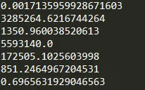
The parameters to be displayed using the "print" command are successfully computed. The last value of 0.69 represents the thermal efficiency of the Otto cycle. This is the same as approximately 69%.

Discussion:

In conclusion, the PV diagram of the engine operating in the Otto cycle for the assumed initial state conditions and geometric parameters is successfully created. The isentropic compression and expansion stages appear as they should with a curved line.

In addition, the thermal efficiency of the engine is also determined to be 69%.

If there were more equally spaced intervals between the start and end crank angles, the plot would appear more smoother.

This python program can be adjusted for different state conditions and geometric parameters of the engine. The program will also comply with different compression ratio values.