Otto Cycle simulation Using Python
Objective: To write a python code that can solve Otto cycle and plot it.
Problem statement: It is necessary to analyze an engine cycle before going to manufacture. Engine air standard cycle is analyzed by plotting its air standard cycle with respect to different variables. It is a time taking procedure to plot a graph by calculating pressure, volume, temperature and constants with respect to air standard cycle. To make the procedure so precise and fast it should be written in a program.
Theory: An Otto cycle is an idealized thermodynamic cycle that describes the functioning of a typical spark ignition piston engine. It is the thermodynamic cycle most commonly found in automobile engines.
The Otto cycle is a description of what happens to a mass of gas as it is subjected to changes of pressure, temperature, volume, addition of heat, and removal of heat. The mass of gas that is subjected to those changes is called the system. The system, in this case, is defined to be the fluid (gas) within the cylinder. By describing the changes that take place within the system, it will also describe in inverse, the system's effect on the environment. In the case of the Otto cycle, the effect will be to produce enough network from the system so as to propel an automobile and its occupants in the environment.
The Otto cycle is constructed as:
Top and bottom of the loop: a pair of quasi-parallel and isentropic processes (frictionless, adiabatic reversible).
Left and right sides of the loop: a pair of parallel isochoric processes (constant volume).
The isentropic process of compression or expansion implies that there will be no inefficiency (loss of mechanical energy), and there be no transfer of heat into or out of the system during that process. The cylinder and piston are assumed to be impermeable to heat during that time. Work is performed on the system during the lower isentropic compression process. Heat flows into the Otto cycle through the left pressurizing process and some of it flows back out through the right depressurizing process. The summation of the work added to the system plus the heat added minus the heat removed yields the net mechanical work generated by the system.
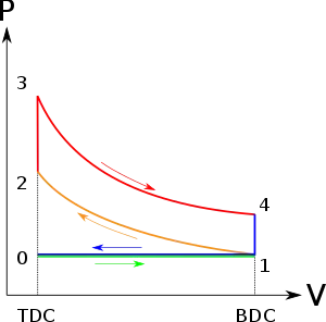
The processes are described by
- Process 0–1 a mass of air is drawn into piston/cylinder arrangement at constant pressure.
- Process 1–2 is an adiabatic (isentropic) compression of the charge as the piston moves from bottom dead centre(BDC) to top dead centre (TDC).
- Process 2–3 is a constant-volume heat transfer to the working gas from an external source while the piston is at top dead centre. This process is intended to represent the ignition of the fuel-air mixture and the subsequent rapid burning.
- Process 3–4 is an adiabatic (isentropic) expansion (power stroke).
- Process 4–1 completes the cycle by a constant-volume process in which heat is rejected from the air while the piston is at bottom dead centre.
- Process 1–0 the mass of air is released to the atmosphere in a constant pressure process.
Volume Trace formula:
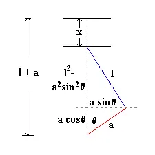
`v/v_c =1+1/2 (r_c-1)[R+1-cosθ-(〖R^2-〖sinθ〗^2)〗^(1/2) ]
The geometric relationship between volume and crank angle given as follows:
v = volume.
v_c = clearance volume.
r_c =compression ratio.
θ = crank angle.
R = connecting rod length (L)/a. crank radius (a) = ½ stroke length(x).
The kinematic equations that are applied in this project are as follows:
Swept volume:
`v_s= π/4* b^2*s`
v_s = swept volume.
b = bore diameter.
s = surface area of cylinder.
Clearance volume:
`v_c= v_s/(r_c-1)`
v_c = clearance volume.
v_s = swept volume.
r_c = clearance volume.
Step-by-step Procedure:
The programme should be such that Input parameters are Bore diameter, Connecting rod length, Stroke length, Compression ratio and the output will be Otto cycle graph.
1.Importing math and plotting library.
#importing libraries
import math
import matplotlib.pyplot as plt
2.Defining Input parameters such as Bore diameter, Connecting rod length, Stroke Length, Compression ratio.
#Geometric parameters (or) Input parameters.
bore = 0.1
stroke = 0.1
con_rod = 0.15
cr = 5
3.Creating a template by defining the engine kinematics like bore, stroke,con_rod,cr,start_crank,end_crank to find the volume trace at a required point.
def engine_kinematics(bore,stroke,con_rod,cr,start_crank,end_crank):
	#engine kinematics
	# crank pin radius
	a = stroke/2
	#constant
	R = con_rod/a
	#volume parameters
	v_s = math.pi*(1/4)*pow(bore,2)*stroke
	v_c = v_s/(cr-1)
	sc = math.radians(start_crank)
	ec = math.radians(end_crank)
	num_values = 50
	dtheta = (ec - sc)/(num_values-1)
	v = []
	for i in range(0,num_values):
		theta = sc + i * dtheta
		term1 = 0.5*(cr-1)
		term2 = R + 1 - math.cos(theta)
		term3 = pow(R,2)-pow(math.sin(theta),2)
		term3 = pow(term3,0.5)
		v.append((1 + term1 * (term2-term3)) * v_c)
	return (v)
4.Giving inputs at Point-1
#inputs
p1 = 101325
t1 = 500
gamma = 1.4
#volume computation
v_s = (math.pi/4)*pow(bore,2)*stroke
v_c = v_s/(cr-1)
v1 = v_c + v_s
5.Giving inputs at Point-2
At point 2 &
From the above equations p2 & t2 can be calculated.
Template is applied with start_crank = 180 & end_crank = 0 and compression volume co-ordinates are calculated as v_compression.
By using volume co-ordinates & above formula pressure co-ordinates are calculated at each crank angle.
#state point 2
v2 = v_c
#p2v2^gamma = p1v1^gamma
p2 = p1*pow(v1,gamma)/pow(v2,gamma)
#p2v2/t2 = p1v1/t1|rhs = p1v1/t1 | lhs = p2v2/t2 | t2 = p2v2/rhs
rhs = p1*v1/t1
t2 = p2*v2/rhs
v_compression = engine_kinematics(bore,stroke,con_rod,cr,180,0)
constant = p1*pow(v1,gamma)
p_compression = []
for v in v_compression:
	p_compression.append(constant/pow(v,gamma))
6.Giving inputs Point-3
As V3 = V2 and input as t3
From p3 is calculated.
Template is applied with start_crank = 0 & end_crank = 1800 and expansion volume co-ordinates are calculated as v_expansion.
By using volume co-ordinates & above formula pressure co-ordinates are calculated at each crank angle.
#state point 3
v3 = v2
t3 = 2300
#p3v3/t3 = p2v2/t2 | rhs = p2v2/t2 |p3 = rhs *t3/v3
rhs = p2 * v2/t2
p3 = rhs * t3/v3
v_expansion = engine_kinematics(bore,stroke,con_rod,cr,0,180)
constant = p3*pow(v3,gamma)
p_expansion = []
for v in v_expansion:
	p_expansion.append(constant/pow(v,gamma))
7.Giving inputs at Point-4
As V4 = V1
From p3 is calculated And from t4 is calculated.
#state point 4
v4 = v1
#p4t4^gamma = p3v3^gamma
p4 = p3 * pow(v3,gamma)/pow(v4,gamma)
#p4v4/t4 = rhs
t4 = p4*v4/rhs
8.Plotting and labelling the points and volume trace.
plt.plot([v2,v3],[p2,p3])
plt.plot(v_compression, p_compression)
plt.plot([v1,v4],[p1,p4])
plt.plot(v_expansion, p_expansion)
plt.xlabel(('VOLUME'),color ='blue')
plt.ylabel(('PRESSURE'),color = 'blue')
plt.show()
Overall code:
#importing libraries
import math
import matplotlib.pyplot as plt
#Geometric parameters (or) Input parameters.
bore = 0.1
stroke = 0.1
con_rod = 0.15
cr = 5
def engine_kinematics(bore,stroke,con_rod,cr,start_crank,end_crank):
	#engine kinematics
	# crank pin radius
	a = stroke/2
	#constant
	R = con_rod/a
	#volume parameters
	v_s = math.pi*(1/4)*pow(bore,2)*stroke
	v_c = v_s/(cr-1)
	sc = math.radians(start_crank)
	ec = math.radians(end_crank)
	num_values = 50
	dtheta = (ec - sc)/(num_values-1)
	v = []
	for i in range(0,num_values):
		theta = sc + i * dtheta
		term1 = 0.5*(cr-1)
		term2 = R + 1 - math.cos(theta)
		term3 = pow(R,2)-pow(math.sin(theta),2)
		term3 = pow(term3,0.5)
		v.append((1 + term1 * (term2-term3)) * v_c)
	return (v)
#inputs
p1 = 101325
t1 = 500
gamma = 1.4
#volume computation
v_s = (math.pi/4)*pow(bore,2)*stroke
v_c = v_s/(cr-1)
v1 = v_c + v_s
#state point 2
v2 = v_c
#p2v2^gamma = p1v1^gamma
p2 = p1*pow(v1,gamma)/pow(v2,gamma)
#p2v2/t2 = p1v1/t1|rhs = p1v1/t1 | lhs = p2v2/t2 | t2 = p2v2/rhs
rhs = p1*v1/t1
t2 = p2*v2/rhs
v_compression = engine_kinematics(bore,stroke,con_rod,cr,180,0)
constant = p1*pow(v1,gamma)
p_compression = []
for v in v_compression:
	p_compression.append(constant/pow(v,gamma))
#state point 3
v3 = v2
t3 = 2300
#p3v3/t3 = p2v2/t2 | rhs = p2v2/t2 |p3 = rhs *t3/v3
rhs = p2 * v2/t2
p3 = rhs * t3/v3
v_expansion = engine_kinematics(bore,stroke,con_rod,cr,0,180)
constant = p3*pow(v3,gamma)
p_expansion = []
for v in v_expansion:
	p_expansion.append(constant/pow(v,gamma))
#state point 4
v4 = v1
#p4t4^gamma = p3v3^gamma
p4 = p3 * pow(v3,gamma)/pow(v4,gamma)
#p4v4/t4 = rhs
t4 = p4*v4/rhs
plt.plot([v2,v3],[p2,p3])
plt.plot(v_compression, p_compression)
plt.plot([v1,v4],[p1,p4])
plt.plot(v_expansion, p_expansion)
plt.xlabel(('VOLUME'),color ='blue')
plt.ylabel(('PRESSURE'),color = 'blue')
plt.show()
Output: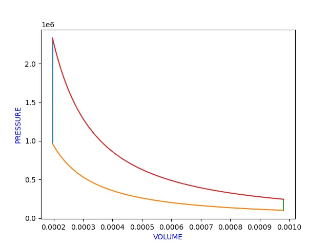
Conclusion:Hence python code is written to solve otto cycle and plot it.