Week 2 Air standard Cycle

Objective:

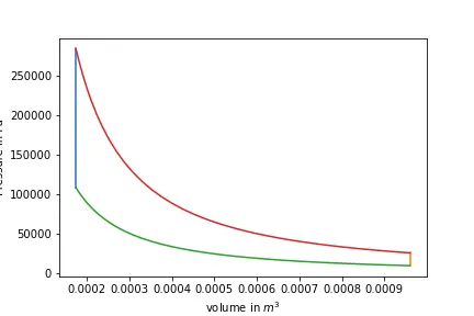
To plot PV diagram for Otto cycle and calculate the ideal otto cycle thermal efficiency using python.

Problem statement:

To plot PV diagram for otto cycle and calculate the thermal efficency and understand the factors affecting the thermal efficiency of otto cycle.

Steps involved:

Understand the Kinematics of IC Engine.

Develop relation between volume change and the crank angle to accurately predict the volume for every crank angle.

Plot the PV diagram in the Pyhton

Predict the Thermal efficeny of ideal otto cycle

The code is written and explained below. The parameters in the code can be altered to study the factors affecting the cycle efficeincy.

Some conclusion can be made such that the efficency is depedent on the compression ratio, temperature of the gas at the inlet and maximum temperature that is reached after heat addition in the engine during power stroke.

'''
Program for Otto cycle

'''

# import libraies

import math
import matplotlib.pyplot as plt

# Initial conditions

p1=10000 # Initial Pressure at state point 1 in Pa
t1=290 # Initial temperature at state point 1 in kelvin
gamma=1.4 # ideal isentropic constant
t3=1500 # Temperature at state point 3 in kelvin
# cylinder geometry details

bore=0.1 # bore diameter in meter
stroke=0.1 # strike length in meter
con_rod=0.2 # length of connecting rod
cr=5.5 #compression ratio of engine

# Calculate the volume

v_s=(math.pi/4)*pow(bore,2)*stroke #stroke volume in m3
v_c=v_s/(cr-1) # clearance volume in m3
v1=v_s+v_c

# caluculate the pressure temperature and volume at state points 2

v2=v_c
# using isentropic compression
p2=p1*pow(v1,gamma)/pow(v2,gamma) # pressure at state point 2 in Pa
 
rhs=p1*v1/t1
t2=p2*v2/rhs # Temeperature in kelvin using ideal gas law
def kinematics_engine(bore,stroke,con_rod,cr,start_crank,end_crank):
    

    a=stroke/2
    R=con_rod/a
    
    v_s=math.pi*(1/4)*pow(bore,2)*stroke
    v_c=v_s/(cr-1)
    sc=math.radians(start_crank)
    ec=math.radians(end_crank)
    numvalues=50
    dtheta=(ec-sc)/(numvalues-1)
    V=[]
    for i in range(0,numvalues):
        
        theta=sc+i*dtheta
        term1=0.5*(cr-1)
        term2=R+1-math.cos(theta)
        term3=pow(pow(R,2)-pow(math.sin(theta),2),0.5)
        
        V.append((1+term1*(term2-term3))*v_c)
        
    return V



V_compression = kinematics_engine(bore,stroke,con_rod,cr,180,0)
constant=p1*pow(v1,gamma)

P_compression=[]
for v in V_compression:
    P_compression.append(constant/pow(v,gamma))


# for state point 3
v3=v2 # Heat addition in Otto cylce is constant volume process cycle
rhs1=p2*v2/t2
p3=t3/v3*rhs1

print(p3>p2) # PRINT ture or false based on the conditions 

# for state point 4 using isentropic expansion
V_expansion = kinematics_engine(bore,stroke,con_rod,cr,0,180)
constant=p3*pow(v3,gamma)

P_expansion=[]
for v in V_expansion:
    P_expansion.append(constant/pow(v,gamma))
                       
                       
v4=v1
p4=p3*pow(v3,gamma)/pow(v4,gamma)
rhs2=p3*v3/t3
t4=p4*v4/rhs2
comp_ratio=v2/v1

thermal_efficiency=1-1/(pow(v1/v2,(gamma-1)))
print(thermal_efficiency) #calculate the thermal efficiency of ideal otto cycle


# plot the graphs
plt.figure()
plt.plot([v2,v3],[p2,p3])
plt.plot([v4,v1],[p4,p1])
plt.plot(V_compression,P_compression)
plt.plot(V_expansion,P_expansion)
plt.xlabel("volume in $m^{3}$ ")
plt.ylabel("Pressure in Pa")

#plt.show()
plt.savefig("otto_cylce_111")