Week 2 Air standard Cycle
Aim:To write the program of an otto cycle in python and plot the graph betwwen the P-V Charactersictics of the otto cycle and finding the thermal efficiency of the engine.
Theory:In the standard otto cycle use for the S I Engine.The otto cycle runs in four proccess,that are
1.Isentropic compression
2.Constant volume heat addition
3.Isentropic expansion
4.Constant volume heat rejection
When the piston moves from Bottom Dead Centre(BDC) to Top Dead Centre(TDC),there will be relatively change in the pressure and volume.We will plot a graph between them to know the changes that take place.The formulae used is:
V/Vc=1+0.5(r_c-1)[R+1-cos(theta)-(R^2-sin^2(theta)^0.5] where,
V=volume at that particular instance
Vc=Cleareance volume
Theta=Crank angle
r_c=Compression ratio
R=Length of connecting rod
The thermal efficiency of the engine is:
Eta=1-1/r_c^(gama-1) where,
Eta=Thermal efficiency of a engine
Procedure:
"""
otto cycle
"""
import math
import matplotlib.pyplot as plt
def engine_kinematics(bore,stroke,con_rod,cr,start_cranck,end_crank):
"""
Engine kinematics
"""
#Geometric parameters
a=stroke/2
R=con_rod/a
#Volume parameters
V_s=math.pi*(1/4)*pow(bore,2)*stroke
V_c=V_s/(cr-1)
sc=math.radians(start_cranck)
ec=math.radians(end_crank)
num_values=50
dtheta=(ec-sc)/(num_values-1)
V=[]
for i in range(0,num_values):
theta=sc+i*dtheta
term1=1/2*(cr-1)
term2=R+1-math.cos(theta)
term3=pow(R,2)-pow(math.sin(theta),2)
term4=pow(term3,1/2)
V.append((1+term1*(term2-term4))*V_c)
return(V)
#Inputs
p1=101525
t1=475
gama=0.8
t3=2100
#Geometric prametres
bore=2/5
stroke=1/5
con_rod=4/25
cr=15
#Volume computation
v_s=(math.pi/4)*pow(bore,2)*stroke
v_c=v_s/(cr-1)
v1=v_c+v_s
#State point 2
v2=v_c
#p2v2^gama=p1v1^gama
p2=p1*pow(v1,gama)/pow(v2,gama)
#p2v2/t2=p1v1/t1 | rhs=p1v1/t1 | p2v2/t2=rhs | t2=p2v2/rhs
rhs=p1*v1/t1
t2=p2*v2/rhs
V_compression=engine_kinematics(bore,stroke,con_rod,cr,180,0)
constant=p1*pow(v1,gama)
P_compression=[]
for v in V_compression:
P_compression.append(constant/pow(v,gama))
#State point 3
v3=v2
#p3v3/t3=p2v2/t2 | rhs=p2v2/t2 | p3=rhs*t3/v3
rhs=p2*v2/t2
p3=rhs*t3/v3
V_expansion=engine_kinematics(bore,stroke,con_rod,cr,0,180)
constant=p3*pow(v3,gama)
P_expansion=[]
for v in V_expansion:
P_expansion.append(constant/pow(v,gama))
#State point 4
v4=v1
#p4v4^gama=p3v3^gama
p4=p3*pow(v3,gama)/pow(v4,gama)
#p4v4/t4=rhs
t4=p4*v4/rhs
plt.plot([v2,v3],[p2,p3])
plt.plot(V_compression,P_compression)
plt.plot(V_expansion,P_expansion)
plt.plot([v4,v1],[p4,p1])
plt.show()
"""
otto cycle
"""
import math
import matplotlib.pyplot as plt
def engine_kinematics(bore,stroke,con_rod,cr,start_cranck,end_crank):
"""
Engine kinematics
"""
#Geometric parameters
a=stroke/2
R=con_rod/a
#Volume parameters
V_s=math.pi*(1/4)*pow(bore,2)*stroke
V_c=V_s/(cr-1)
sc=math.radians(start_cranck)
ec=math.radians(end_crank)
num_values=50
dtheta=(ec-sc)/(num_values-1)
V=[]
for i in range(0,num_values):
theta=sc+i*dtheta
term1=1/2*(cr-1)
term2=R+1-math.cos(theta)
term3=pow(R,2)-pow(math.sin(theta),2)
term4=pow(term3,1/2)
V.append((1+term1*(term2-term4))*V_c)
return(V)
#Inputs
p1=101525
t1=475
gama=0.8
t3=2100
#Geometric prametres
bore=2/5
stroke=1/5
con_rod=4/25
cr=15
#Volume computation
v_s=(math.pi/4)*pow(bore,2)*stroke
v_c=v_s/(cr-1)
v1=v_c+v_s
#State point 2
v2=v_c
#p2v2^gama=p1v1^gama
p2=p1*pow(v1,gama)/pow(v2,gama)
#p2v2/t2=p1v1/t1 | rhs=p1v1/t1 | p2v2/t2=rhs | t2=p2v2/rhs
rhs=p1*v1/t1
t2=p2*v2/rhs
V_compression=engine_kinematics(bore,stroke,con_rod,cr,180,0)
constant=p1*pow(v1,gama)
P_compression=[]
for v in V_compression:
P_compression.append(constant/pow(v,gama))
#State point 3
v3=v2
#p3v3/t3=p2v2/t2 | rhs=p2v2/t2 | p3=rhs*t3/v3
rhs=p2*v2/t2
p3=rhs*t3/v3
V_expansion=engine_kinematics(bore,stroke,con_rod,cr,0,180)
constant=p3*pow(v3,gama)
P_expansion=[]
for v in V_expansion:
P_expansion.append(constant/pow(v,gama))
#State point 4
v4=v1
#p4v4^gama=p3v3^gama
p4=p3*pow(v3,gama)/pow(v4,gama)
#p4v4/t4=rhs
t4=p4*v4/rhs
plt.plot([v2,v3],[p2,p3])
plt.plot(V_compression,P_compression)
plt.plot(V_expansion,P_expansion)
plt.plot([v4,v1],[p4,p1])
plt.show()
#Efficiency of a otto cycle
eta=1-(1/cr)^(gama-1)
print(eta)
By using the above the code we can create the plot of the otto cycle of P-V characteristics and find the efficiency of a otto cycle.
Results:The air standard otto cycle plot for P-V Characteristics: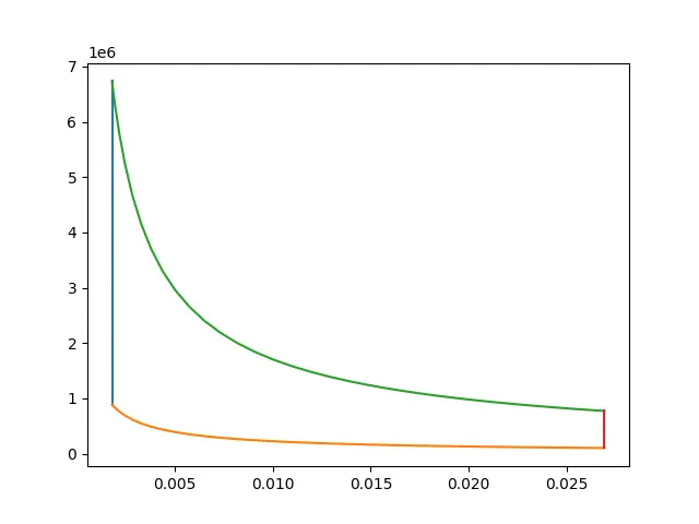
Efficiency of otto cycle is =0.71 or 71%
Conculsion:We have umderstood the working of a otto cycle and plotted the graphs between P-V Characteristics,calculated the value of thermal efficiency.