Week 2 Air standard Cycle

Objective:

Program to create a PV diagram for otto cycle and calculate the thermal efficiency of the engine.

In this report, we will solve and write a code to simulate otto cycle to create the PV diagram. We will also find the thermal efficiency of the engine. We calculate state variables at four stages then plot the PV diagram.

Otto cycle:

It is a thermodynamic cycle that is commonly found in automobile engines which generally describes function of a spark ignition piston engine. It describes the mass of gas when it is subjected to change in pressure, temperature, and volume.

Otto cycle is developed from a pair of quasi parallel and isentropic processes, parallel constant volume.

Otto cycle generally consists of 4 processes:

1-2: Isentropic Compression

2-3: Constant volume heat transfer

3-4: Isentropic expansion

4-1: Constant volume heat rejection

Otto cycle uses the thermodynamic equations that are essential to simulate the PV diagram

Governing Equations:

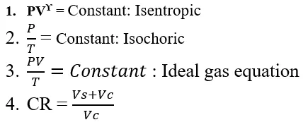
Where,

P = pressure Vc = Clearance volume

V= Volume

T = temperature(kelvin) `gamma`= 1.4 : ratio of specific heats

Vs = Swept Volume

To complete our otto cycle simulation we need to have the volume trace of the cycle. To get that we need to solve a particular equation which describes the relationship between crank angle and volume inside the combustion chamber.

The Volume change in the combustion chamber w.r.t crank angle is given by:

^where:

V = Volume at angle the piston makes

Vc = Clearance volume

CR =Compression ratio

R = Ration of length of connect rod to crank pin radius

Crank pin radius (a) = stroke/2

a =stroke/2 R = con_rod/a

Code:

To solve the otto cycle and simulate the PV diagram we need to define a function where we define the engine kinematics with parameters and the parameters.

This function helps to calculate the pressures corresponding to volumes at various crank angles for compression and expansion strokes.

The angles vary from 0 to 180 in both compression and expansion process.

^{Function inputs:}

^{bore, stroke, con_rod, cr, start crank angel, end crank angle}

# Engine Kinematics

import math

#Geometric parameters

bore = 0.1
stroke = 0.1
con_rod = 0.15
cr = 12
a = stroke/2
R = con_rod/a

#Volume computation
v_s = (math.pi/4)*pow(bore,2)*stroke
v_c = v_s/(cr-1)

theta = math.radians(0)

term1 = 0.5*(cr-1)
term2 = R+1-math.cos(theta)
term3 = pow(R,2)-pow(math.sin(theta),2)
term3 = pow(term3,0.5)

V = (1+ term1*(term2-term3))*v_c

^Inputs:

^{We provide the following inputs to solve the otto cycle}

^{p1 = 101325 pascals}

^{t1 = 500 kelvin}

^{gamma = 1.4}

^{t3 = 2300 kelvin}

^{Geometric parameters:}

^{bore = 0.1}

^{stroke = 0.1}

^{con_rod = 0.15}

^{cr = 8}

^{We define the state variables and apply the governing equations to calculate the pressure and volume at each stage. The function which we have defined will calculate volume as function of angle and its related pressure so that we can plot the PV diagram.}

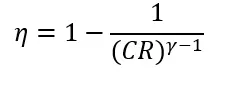
^{The thermal efficiency of the engine is calculated by:}

^Code:

#Air standard Cycle

import math
import matplotlib.pyplot as plt 

def Engine_kinematics(bore,stroke,con_rod,cr,start_crank,end_crank):
	# Engine Kinematics

	#Geometric parameters

	a = stroke/2
	R = con_rod/a

	#Volume computation
	v_s = (math.pi/4)*pow(bore,2)*stroke
	v_c = v_s/(cr-1)

	sc = math.radians(start_crank)
	ec = math.radians(end_crank)

	num_values = 50
	dtheta = (ec-sc)/(num_values-1)
	V = []

	for i in range(0,num_values):
		theta = sc + i*dtheta

		term1 = 0.5*(cr-1)
		term2 = R+1-math.cos(theta)
		term3 = pow(R,2)-pow(math.sin(theta),2)
		term3 = pow(term3,0.5)

		V.append((1 + term1*(term2-term3))*v_c)
	return V

		


#Inputs
p1 = 101325
t1 = 500
gamma = 1.4
t3 = 2300

#Geometric parameters
bore = 0.1
stroke = 0.1
con_rod = 0.15
cr = 8

#Volume computation
v_s = (math.pi/4)*pow(bore,2)*stroke
v_c = v_s/(cr-1)
v1 = v_c + v_s

#state point 2
v2 = v_c

#p2v2^gamma = p1v1^gamma
p2 = p1*pow(v1,gamma)/pow(v2,gamma)

#p2v2/t2 = p1v1/t1 | rhs = p1v1/t1 | p2v2/t2 = rhs | t2 = p1v2/rhs
rhs = p1*v1/t1
t2 = p2*v2/rhs
V_compression = Engine_kinematics(bore, stroke, con_rod, cr, 180, 0)

constant = p1*pow(v1,gamma)
P_compression = []

for v in V_compression:
	P_compression.append(constant/pow(v,gamma))

#state point 3
v3 = v2

#p3v3/t3 = p2v2/t2 |rhs = p2v2/t2 | p3 = rhs*t3/v3

rhs = p2*v2/t2
p3 = rhs*t3/v3

V_expansion = Engine_kinematics(bore, stroke, con_rod, cr, 0, 180)

constant = p3*pow(v3,gamma)
P_expansion = []

for v in V_expansion:
	P_expansion.append(constant/pow(v,gamma))


#state point 4
v4 = v1

#p4v4^gamma = p3v3^gamma

p4 = p3*pow(v3,gamma)/pow(v4,gamma)

#p4v4/t4 = rhs

t4 = p4*v4/rhs

plt.plot([v2,v3],[p2,p3])
plt.plot(V_compression,P_compression)
plt.plot(V_expansion,P_expansion)
plt.plot([v4,v1],[p4,p1])
plt.show()

#Thermal Efficiency 

n = 1-(pow(cr,(1-gamma)))
print(n)

Results:

PV Diagram:

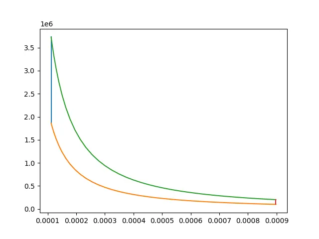
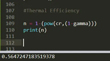
Thermal Efficiency of the engine: 56.47%

Conclusion:

By the help of the above code we have simulated the otto cycle and determined the thermal efficiency of the engine.

The thermal efficiency of the engine is found to be 56.47% for the inputs we have given.