Week 2 Air standard Cycle

Aim

To write a Python code that can solve the otto cycle such that it will generate the PV diagram for the given conditions and also compute the thermal efficiency for the same set of initial conditions.

Algorithm

1. Fix the state variables like atmospheric pressure and temperature of the working condition.
2. Fix the inputs which are required in the calculation of the different parameters in the state variable like gamma and value of temperature at point 3.
3. Now provide the value of parametric values of the IC engine like bore radius, stroke, etc so that clearance volume and swept volume can be calculated.
4. Now use the clearance volume and swept volume to determine the values at state point 1 and 2.
5. Determine all the state variable points of the PV diagram.
6. Create a function that will generate the actual curve during the expansion and compression process using parametric values of stroke, bore radius, etc.
7. For straight lines use the plot command to get the total PV curve for the given condition in an IC engine.

Python code

# otto cycle program
import math
import matplotlib.pyplot as plt

#function for returning the value of volume at every point of the adiabatic process
def engine_kinematics(bore,stroke,c_rod,cr,start_crank,end_crank):

	a=stroke/2
	R=c_rod/a

	# Volumetric parameters
	V_s=math.pi*(1/4)*pow(bore,2)*stroke
	V_c=V_s/(cr-1)
    
    # to get the parabolic curves between the state points
	sc=math.radians(start_crank)
	ec=math.radians(end_crank)

	n_values=50
	dtheta=(ec-sc)/(n_values-1)

	V=[]
	for i in range(0,n_values):
		theta=sc + i*dtheta
		
		term1=0.5*(cr-1)
		term2=R + 1 - math.cos(theta)
		term3=pow(R,2)-pow(math.sin(theta),2)
		term4=pow(term3,0.5)

		V.append((1 + term1*(term2-term4))*V_c)
		
	return V # returns the value of V within the program when called


#inputs
p1=101325 # Pressure at state point 1 in Pascal
t1=500 # Temperature at state point 1 in Kelvin
gamma=1.4
t3=2300 #Temperature at state point 3 in Kelvin

#geometric parameters
bore=0.1
stroke=0.1
c_rod=0.16 #connecting rod
cr=10 #compression ratio

# volume computation
v_s=(math.pi/4)*pow(bore,2)*stroke
v_c=v_s/(cr-1)
v1=v_c+v_s

#At state point 2
v2=v_c

# p2v2^gamma=p1v1^gamma
p2=p1*pow(v1,gamma)/(pow(v2,gamma))

# p2v2/t2=p1v1/t1 | rhs=p1v1/t1 | from the ideal gas equation| p2v2/t2=rhs 
rhs=p1*v1/(t1)
t2=p2*v2/rhs

V_compression=engine_kinematics(bore,stroke,c_rod,cr,180,0 )

constant=p1*pow(v1,gamma)

P_compression=[]

for v in V_compression:
	P_compression.append(constant/pow(v,gamma))


# At state point 3
v3=v2

# for pressure p3v3/t3=rhs=p2v2/t2|
rhs= p2*v2/t2
p3=rhs*t3/v3


V_expansion=engine_kinematics(bore,stroke,c_rod,cr,0,180 )

constant=p3*pow(v3,gamma)

P_expansion=[]

for v in V_expansion:
	P_expansion.append(constant/pow(v,gamma))

# at state point 4
v4=v1

#p4v4^gamma=p3v3^gamma
p4=p3*pow(v3,gamma)/pow(v4,gamma)

# rhs is a constant
t4=p4*v4/rhs

# Thermal Efficency calculation
nu_t2=1-pow((v2/v1),(gamma-1))
nu_t1=1-pow(cr,(1-gamma))
print("Thermal effeciency of the engine is")
print(nu_t1*100)
print(v1,v2,v3,v4)
print(p1,p2,p3,p4)

#ploting section
plt.plot([v2,v3],[p2,p3])
plt.plot(V_compression,P_compression)
plt.plot(V_expansion,P_expansion)
plt.plot([v4,v1],[p4,p1])
plt.xlabel('Volume')
plt.ylabel('Pressure')
plt.show()

Working of code

1. Various constants, as well as a state variable, is fixed as per the algorithm given to determine various parameters of all other state variable points in the PV diagram.
2. The code uses the normal equations as well as parametric formulas to get the required values so that the calculation can be executed further.
3. Once this is determined, the code uses the equation of the curves of a PV diagram to get the values of other state points in the graph.
4. Now the code plots all these points in a graph to get a general idea of the area of the curve generated in the given condition of the IC engine.
5. Now for the final curves that will join the four-state points that are found earlier a function has to be created which will plot the required curve.
6. This function will take inputs of bore radius, stroke length, connecting rod length, compression ratio as well as the starting and the end angle of the crank- piston arrangement.
7. The function is based on the mathematical formula that defines the nature of the curve during the expansion and compression process.
8. The code introduces this function in the main program to get the actual curves joining the various state points instead of the straight lines.
9. Plot command in the code connects the rest of the points using plot command to get a straight line as is known from the mathematical derivation of the pressure vs volume curve for an IC engine.

Errors and solutions

• The requirement of temperature for the 3rd state point- This was resolved by fixing the value of this variable in the program itself.
• The straight lines connecting 2-3 and 4-1 in the graph- This was solved using the plot command for straight lines so that the curve generated is a fully closed curve.
• Syntax errors- Small syntax errors regarding the introduction of the various variables in the newly inserted function were found which was corrected using the help and support in the python help manual.

Output

• The final PV diagram using this program is

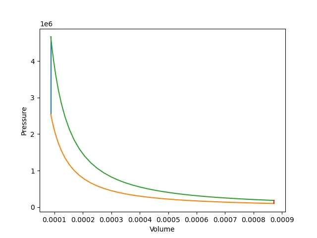
• The efficiency of the engine is 60.189282944650266

Conclusion

The PV diagram of the Otto cycle for IC engine has been successfully generated using this Python code and also the thermal efficiency of the given condition has been successfully calculated and displayed by the program code