Week 2 Air standard Cycle

ENGINE KINEMATICS – THE OTTO CYCLE SIMULATOR

Objectives

• To write a python code and generate the PV diagram of the Otto cycle.
• To calculate the thermal efficiency of the engine.

Problem Statement

An Otto cycle is an ideal thermodynamic cycle that describes the working of an automobile engine, spark ignition piston type in particular. It is a combination of four thermodynamic processes and is used to study the overall functioning of an engine from a thermodynamic point of view. The PV and TS diagrams of the Otto cycle are as follows.

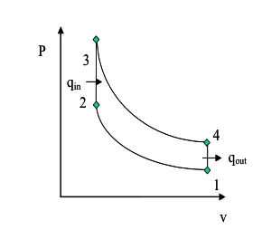
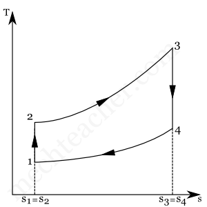
The processes involved are as follows

Process 1-2: Isentropic compression

Process 2-3: Isochoric heat addition

Process 3-4: Isentropic expansion

Process 4-1: Isochoric heat rejection

The thermal efficiency of the Otto cycle is calculated as follows.

`η=1- 1/(〖cr〗^γ-1)`

In this formula, cr stands for the compression ratio, and the constant stands for the ratio of specific heats, a non-dimensional quantity.

Also, the variation of pressure with volume in the isentropic process follows the principle To consider this equation, the volume in these processes is calculated using the formula below.

`V/V_c =1+ 1/2×(cr-1)×[R+1-cos⁡θ- (R^2- 〖sin⁡θ〗^2 )^(1⁄2)]`

Solution Procedure

• Initially, the math, plotting, and NumPy libraries are imported so that calculations and plotting operations can be performed.
• A new function is defined under the name engine kinematics which uses certain parameters like dimensions of bore, stroke, length of connecting rod, compression ratio, and the crank angles.
• Required geometric parameters and volume parameters namely swept volume and compressed volume is calculated.
• To generate a smooth curve, a set of values would be required. Accordingly, a range of angles is defined using the linspace function and stored in an array.
• Now, to calculate the volume using equation 2, a for loop is defined to input the range of angles. Also, the formula is broken down into three terms and added together later by storing it in a temporary variable. Append function is used to add values into an array. The function definition ends with a return statement which is used to return the values later.
• Now, initial temperature and pressure conditions are defined along with the values of gamma. Also, the highest temperature in the process is defined. In addition to this, the geometric parameters used in the function are also defined.
• Now, the pressure, volume, and temperature at four state points are calculated using the graph and certain equations.
• In addition to this, the function defined initially is used at state points 2 and 4 since these are isentropic processes. An array of the volume is created initially, and the function call is assigned to it. Later, a pressure array is created and a for loop is used to calculate and store the values of the corresponding pressure values. Thus, all of the required values are calculated.
• Using the formula in equation 1, the thermal efficiency of the overall system is calculated.
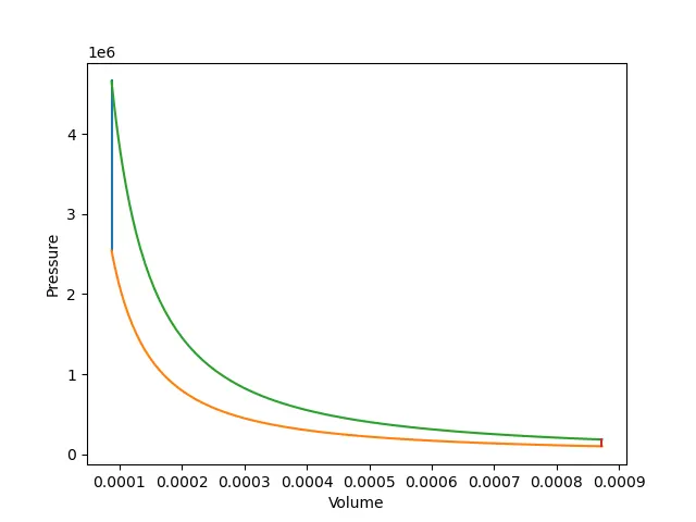
• Finally, code is written for the plotting of every process, thus generating the PV diagram.
• The code is as follows.

# Otto Cycle Simulator

import math
import matplotlib.pyplot as plt 
import numpy as np 

# Defining a function to calculate actual volume and related parameters
def engine_kinematics(bore,stroke,con_rod,cr,start_crank,end_crank):
	#Inputs
	a = stroke/2
	R = con_rod/a

	# Volume parameters
	v_s = (math.pi/4)*pow(bore,2)*stroke
	v_c = v_s/(cr-1)
	
	angles = np.linspace(math.radians(start_crank),math.radians(end_crank),100)

	V = []

	for theta in angles:
		term1 = 0.5*(cr-1)
		term2 = R + 1 - math.cos(theta)
		term3 = pow(R,2) - pow(math.sin(theta),2)
		term3 = pow(term3,0.5)
		x = (1 + term1*(term2-term3))*v_c
		V.append(x)

	return V 

# Inputs
p1 = 101325
t1 = 500
gamma = 1.4
t3 = 2300

# Geometric Parameters
bore = 0.1
stroke = 0.1
con_rod = 0.15
cr = 10

# Volume Computation
v_s = (math.pi/4)*pow(bore,2)*stroke
v_c = v_s/(cr-1)
v1 = v_c + v_s

# State point 2
v2 = v_c

# Isentropic compression | p2v2^gamma = p1v1^gamma | 
p2 = p1*pow(v1,gamma)/pow(v2,gamma)

# p2v2/t2 = p1v1/t1 | rhs = p1v1/t1
rhs = p1*v1/t1
t2 = (p2*v2)/rhs

# Function is used to calculate the values of pressure and volume during compression
V_compression = engine_kinematics(bore,stroke,con_rod,cr,180,1)  # Angles vary from 180 to 1 because piston moves upwards from BDC to TDC
# pv^gamma = constant
constant = p1*pow(v1,gamma)
P_compression = []
for v in V_compression:
	P_compression.append(constant/pow(v,gamma))

# State point 3
v3 = v2

# Constant volume heat addition | p3v3/t3 = p2v2/t2 | rhs = p2v2/t2
# rhs is same throughout the process since Otto cycle is a closed loop
p3 = (t3*rhs)/v3

# State point 4
v4 = v1

# Isentropic expansion | p3v3^gamma = p4v4^gamma |
p4 = p3*pow(v3,gamma)/pow(v4,gamma)

# p4v4/t4 = p3v3/t3 | rhs = p3v3/t3
t4 = (p4*v4)/rhs

# Function is used again to calculate the values of pressure and volume during expansion
V_expansion = engine_kinematics(bore,stroke,con_rod,cr,1,180)  # Angles vary from 1 to 180 because piston moves downwards from TDC to BDC
P_expansion = []
constant = p3*pow(v3,gamma)
for v in V_expansion:
	P_expansion.append(constant/pow(v,gamma))

# Thermal efficiency
Efficiency = 1 - (1/(pow(cr,gamma) - 1))
print(Efficiency)

# Plotting graphs
plt.plot([v2,v3],[p2,p3])
plt.plot(V_compression,P_compression)
plt.plot(V_expansion,P_expansion)
plt.plot([v4,v1],[p4,p1])
plt.xlabel('Volume')
plt.ylabel('Pressure')
plt.savefig('Otto Cycle')
plt.show()

Results

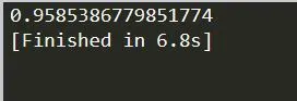
The thermal efficiency of the system is obtained as follows.

The PV diagram of the system is obtained as follows

Discussions

Instead of using a for loop to define and store the values of angles, linspace function is used which reduces the number of lines of code and makes the code easier to read and understand. Using a function makes the whole code look generic and it can be used to calculate required values and plot corresponding graphs for any set of inputs.