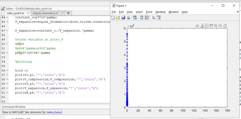
Error 5

1. In this error graph is not properly observed,error found to be in engine kinematics
   program wher plot command is given in 'function' command.
   so, removing plot command thus error is fixed
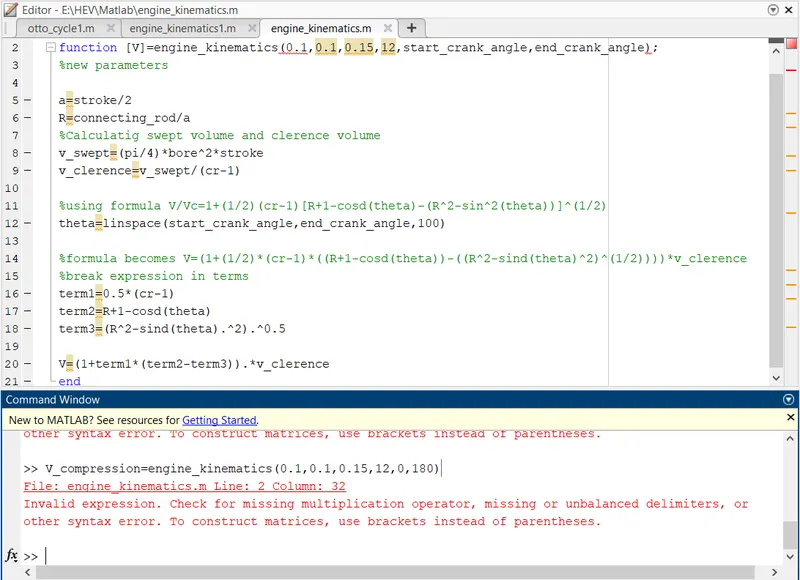
Error 4

1. In this error, instead of input parameter in line 2 input values are written.
   By writing input parameter,error is resolved.
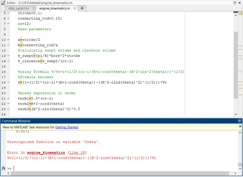
Error 3

1. Maintain the syntax as sind^2(theta).
   Hence issue is reoslved.
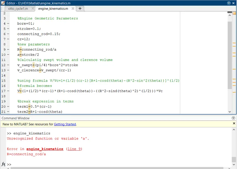
Error 2

1. In this error we have to first define the 'a'.
   then to find 'R',SO maintain proper seqeuence.
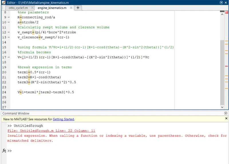
Error 1
1. In this error wrong parenthesis is used i.e '[]'.
   so,to correct the error replace it with'()'.
2. Also check the number of open and close braces,to correct the mismatched delimeters.
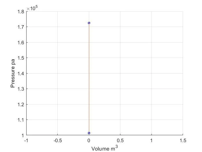
Process 4-1:constant volume heat rejection
            adiabatic process takes place as pressure is decreased and heat rejection
            result in loss of energy.
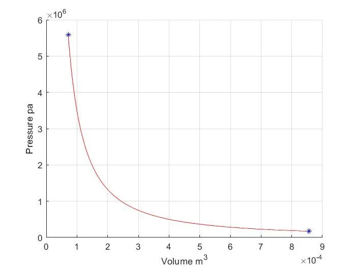
Process 3-4:isentropic expansion
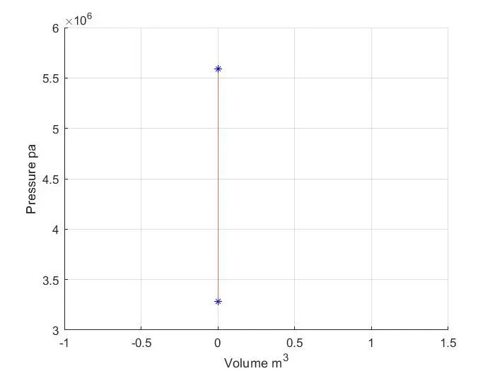
 Process 2-3:constant volume heat addition
             adaibatic process takes place as pressure is increased and heat addition
             takes place.
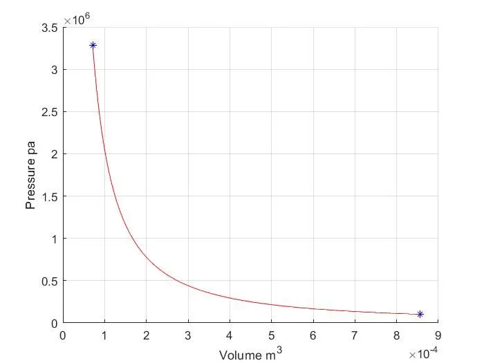
Process 1-2:iscentropic compression
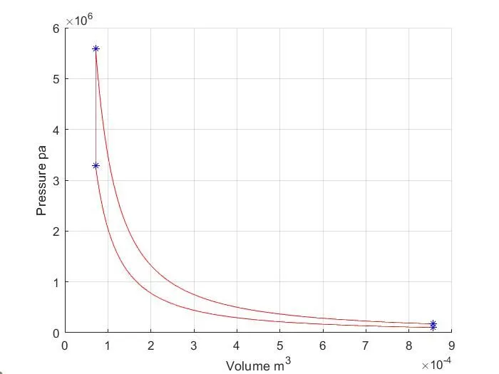
Output:

This is PV diagram for Air standard Otto Cycle

Process 1-2:iscentropic compression
Process 2-3:constant volume heat addition
Process 3-4:iscentropic expansion
Process 4-1:constant volume heat rejection
Output:

gamma =1.4000

t3 = 2300

p1 = 101325

t1 = 500

v_swept =7.8540e-04

v_clerence =7.1400e-05

v1 =8.5680e-04

v2 =7.1400e-05

p2 =3.2853e+06

v3 =7.1400e-05

p3 = 5593140

v4 = 8.5680e-04

p4 = 1.7251e+05

efficiency_otto_cycle =62.9893

This is the efficiency of Otto cycle.
%Engine Geometric Parameters using function

function [V]=engine_kinematics(bore,stroke,connecting_rod,cr,start_crank_angle,end_crank_angle);

%new parameters

a=stroke/2;
R=connecting_rod/a;
%Calculatig swept volume and clerence volume
v_swept=(pi/4)*bore^2*stroke;
v_clerence=v_swept/(cr-1);

%using formula V/Vc=1+(1/2)(cr-1)[R+1-cosd(theta)-(R^2-sin^2(theta))]^(1/2)
theta=linspace(start_crank_angle,end_crank_angle,100);


%formula becomes V=(1+(1/2)*(cr-1)*((R+1-cosd(theta))-((R^2-sind(theta)^2)^(1/2))))*v_clerence
%break expression in terms
term1=0.5*(cr-1);
term2=R+1-cosd(theta);
term3=(R^2-sind(theta).^2).^0.5;

V=(1+term1*(term2-term3)).*v_clerence;

end

%this program is to find how compression process takes place inside the cylinder
%this program is to find out how expansion process take place inside the cylinder
%by using  this function command, we can directly put the tempelate in main command in order to shorten the main program.
%Program for Air Standard Otto Cycle, Plot PV diagram.

%Inputs
gamma=1.4
t3=2300

%State Variables
p1=101325
t1=500

%Engine Geometric Parameters
bore=0.1;
stroke=0.1;
connecting_rod=0.15;
cr=12;

%Calculatig swept volume and clerence volume
v_swept=(pi/4)*bore^2*stroke
v_clerence=v_swept/(cr-1)

v1=v_swept+v_clerence
v2=v_clerence

%State variable at point_2
%p2v2^gamma=p1v1^gamma
%p2=p1*(v1/v2)^gamma
p2=p1*cr^gamma

%p2v2/t2=p1v1/t1
t2=(p2*v2*t1)/(p1*v1);

constant_c=p1*v1^gamma;
V_compression=engine_kinematics(bore,stroke,connecting_rod,cr,180,0);

P_compression=constant_c./V_compression.^gamma;


%state Variable at point_3
v3=v2
%p3v3/t3=p2v2/t2
p3=p2*t3/t2

constant_c=p3*v3^gamma;
V_expansion=engine_kinematics(bore,stroke,connecting_rod,cr,0,180);

P_expansion=constant_c./V_expansion.^gamma;

%state variable at point_4
v4=v1
%p4v4^gamma=p3v3^gamma
p4=p3*(v3/v4)^gamma

%efficiency of Otto cycle
efficiency_otto_cycle=(1-(1/cr.^(gamma-1)))*100


%plotting
%otto cycle PV diagram

figure(1)
hold on
plot(v1,p1,'*','color','b')
plot(V_compression,P_compression,'color','r')
plot(v2,p2,'*','color','b')
plot(v3,p3,'*','color','b')
plot(V_expansion,P_expansion,'color','r')
plot(v4,p4,'*','color','b')
plot([v2,v3],[p2,p3])
plot([v4,v1],[p4,p1])
xlabel('Volume m^3')
ylabel('Pressure pa')
grid on

%process 1-2 isentropic compression PV diagram
figure(2)
hold on
plot(v1,p1,'*','color','b')
plot(V_compression,P_compression,'color','r')
plot(v2,p2,'*','color','b')
xlabel('Volume m^3')
ylabel('Pressure pa')
grid on

%process 2-3 constant vol. heat addition PV diagram
figure(3)
hold on
plot(v2,p2,'*','color','b')
plot([v2,v3],[p2,p3])
plot(v3,p3,'*','color','b')
xlabel('Volume m^3')
ylabel('Pressure pa')
grid on

%process 3-4 isentropic expansion PV diagram
figure(4)
hold on
plot(v3,p3,'*','color','b')
plot(V_expansion,P_expansion,'color','r')
plot(v4,p4,'*','color','b')
xlabel('Volume m^3')
ylabel('Pressure pa')
grid on

%process 4-1 constant vol. heat rejection PV diagram
figure(5)
hold on
plot(v4,p4,'*','color','b')
plot([v4,v1],[p4,p1])
plot(v1,p1,'*','color','b')
xlabel('Volume m^3')
ylabel('Pressure pa')
grid on