Week 12 - Validation studies of Symmetry BC vs Wedge BC in OpenFOAM vs Analytical H.P equation
Continuining from the previous challenge, the script creating the blockMeshDict file was used to get the file for 10, 25 and 45 deg wedge angle.
The blockMeshDict creater script is as below:-
% Matlab script for generating the blockMeshDict file given wedge angle
clear all
close all
clc

%% Properties declaration
% User input wedge Angle
theta = input(' Enter the value of wedge angle in degrees: ');

% Assumed Diameter of the pipe
D = input(' Enter the value of pipe diameter in m: ');

%L = 0.06*Re*D; % Length of the pipe

% User input Length
L = input('\n Enter the value of Length of Pipe in m: ');
% Radius of the Pipe
R=D/2;

% No. of cells along the radial direction
N1 = 50;
% No. of cells along the circumferential direction
N2 = 1;
% No. of cells along the length direction
N3 = 200;

%% Wedge fomation
% Center of the pipe
v0 = [0 0 0];
% Vertices on the circumference of the pipe
vc01 = [0 R*cosd(theta/2) -R*sind(theta/2)];
vc02 = [0 R*cosd(theta/2) R*sind(theta/2)];

% Corresponding Vertices on the other side of the pipe
v1 = [L 0 0];
vc11 = [L R*cosd(theta/2) -R*sind(theta/2)];
vc12 = [L R*cosd(theta/2) R*sind(theta/2)];


% Header of the file
file_type=' FoamFile';
% Header Dictionary
Dl1='{';
Dl2='    version     2.0;';
Dl3='    format      ascii;';
Dl4='    class       dictionary;';
Dl5='    object      blockMeshDict;';
Dl6='}';
% Creating file
file = fopen('blockMeshDict','wt');

fprintf(file,'%s\n',file_type);
fprintf(file,'%s\n',Dl1);
fprintf(file,'%s\n',Dl2);
fprintf(file,'%s\n',Dl3);
fprintf(file,'%s\n',Dl4);
fprintf(file,'%s\n',Dl5);
fprintf(file,'%s\n',Dl6);
fprintf(file,'\n');

fprintf(file,'%s\n','convertToMeters 1;');
%% Geometry Declaration
% Declaring the Vertices
fprintf(file,'%s\n','vertices');
fprintf(file,'%s\n','(');

fprintf(file,'%s (%f %f %f) \n',blanks(5),v0(1),v0(2),v0(3)); % vertex 0
fprintf(file,'%s (%f %f %f) \n',blanks(5),v1(1),v1(2),v1(3)); % vertex 1
fprintf(file,'%s (%f %f %f) \n',blanks(5),vc01(1),vc01(2),vc01(3)); % vertex 2
fprintf(file,'%s (%f %f %f) \n',blanks(5),vc11(1),vc11(2),vc11(3)); % vertex 3
fprintf(file,'%s (%f %f %f) \n',blanks(5),vc02(1),vc02(2),vc02(3)); % vertex 4
fprintf(file,'%s (%f %f %f) \n',blanks(5),vc12(1),vc12(2),vc12(3)); % vertex 5
fprintf(file,'%s\n',');');
fprintf(file,'\n');

% Declaring the Wedge block
fprintf(file,'%s\n','blocks');
fprintf(file,'%s\n','(');
fprintf(file,'%s %s %d %d %d %s\n',blanks(5),'hex (0 2 4 0 1 3 5 1) (',N1,N2,N3,') simpleGrading (0.8 1 1)');
fprintf(file,'%s\n',');');
fprintf(file,'\n');

% Declaring the arc edges
fprintf(file,'%s\n','edges');
fprintf(file,'%s\n','(');
fprintf(file,'%s arc 2 4 (%f %f %f) \n',blanks(5),0,R,0);
fprintf(file,'%s arc 3 5 (%f %f %f) \n',blanks(5),L,R,0);
fprintf(file,'%s \n',');');
fprintf(file,'\n');

% Declaring the boundary names
fprintf(file,'%s\n','boundary');
fprintf(file,'%s\n','(');
% Input Flow face
fprintf(file,'%s %s \n',blanks(5),'inlet_flow');
fprintf(file,'%s %s \n',blanks(5),'{');
fprintf(file,'%s %s \n',blanks(10),'type patch;');
fprintf(file,'%s %s \n',blanks(10),'faces');
fprintf(file,'%s %s \n',blanks(10),'(');
fprintf(file,'%s %s \n',blanks(15),'(0 2 4 0)');
fprintf(file,'%s %s \n',blanks(10),');');
fprintf(file,'%s %s \n',blanks(5),'}');

% Outlet flow face
fprintf(file,'%s %s \n',blanks(5),'outlet_flow');
fprintf(file,'%s %s \n',blanks(5),'{');
fprintf(file,'%s %s \n',blanks(10),'type patch;');
fprintf(file,'%s %s \n',blanks(10),'faces');
fprintf(file,'%s %s \n',blanks(10),'(');
fprintf(file,'%s %s \n',blanks(15),'(1 3 5 1)');
fprintf(file,'%s %s \n',blanks(10),');');
fprintf(file,'%s %s \n',blanks(5),'}');

% Right Side face
fprintf(file,'%s %s \n',blanks(5),'right');
fprintf(file,'%s %s \n',blanks(5),'{');
fprintf(file,'%s %s \n',blanks(10),'type wedge;');
fprintf(file,'%s %s \n',blanks(10),'faces');
fprintf(file,'%s %s \n',blanks(10),'(');
fprintf(file,'%s %s \n',blanks(15),'(0 1 5 4)');
fprintf(file,'%s %s \n',blanks(10),');');
fprintf(file,'%s %s \n',blanks(5),'}');

% Left Side face
fprintf(file,'%s %s \n',blanks(5),'left');
fprintf(file,'%s %s \n',blanks(5),'{');
fprintf(file,'%s %s \n',blanks(10),'type wedge;');
fprintf(file,'%s %s \n',blanks(10),'faces');
fprintf(file,'%s %s \n',blanks(10),'(');
fprintf(file,'%s %s \n',blanks(15),'(0 2 3 1)');
fprintf(file,'%s %s \n',blanks(10),');');
fprintf(file,'%s %s \n',blanks(5),'}');

% Pipe Curvature
fprintf(file,'%s %s \n',blanks(5),'curvature');
fprintf(file,'%s %s \n',blanks(5),'{');
fprintf(file,'%s %s \n',blanks(10),'type wall;');
fprintf(file,'%s %s \n',blanks(10),'faces');
fprintf(file,'%s %s \n',blanks(10),'(');
fprintf(file,'%s %s \n',blanks(15),'(2 3 5 4)');
fprintf(file,'%s %s \n',blanks(10),');');
fprintf(file,'%s %s \n',blanks(5),'}');

% Axis
fprintf(file,'%s %s \n',blanks(5),'axis_coor');
fprintf(file,'%s %s \n',blanks(5),'{');
fprintf(file,'%s %s \n',blanks(10),'type empty;');
fprintf(file,'%s %s \n',blanks(10),'faces');
fprintf(file,'%s %s \n',blanks(10),'(');
fprintf(file,'%s %s \n',blanks(15),'(0 1 1 0)');
fprintf(file,'%s %s \n',blanks(10),');');
fprintf(file,'%s %s \n',blanks(5),'}');
fprintf(file,'%s \n',');');
fprintf(file,'\n');


fprintf(file,'%s \n','mergePatchPairs');

fprintf(file,'%s \n','(');
fprintf(file,'%s \n',');');

fprintf(file,'\n');

%% File writing closure
fclose(file);
The boundary condition files were modified for symmetry and wedge.
Below is (10deg) one of the files used to carry out the simulation:-
The blockMeshDict file:-
 FoamFile
{
    version     2.0;
    format      ascii;
    class       dictionary;
    object      blockMeshDict;
}

convertToMeters 1;
vertices
(
      (0.000000 0.000000 0.000000)
      (3.000000 0.000000 0.000000)
      (0.000000 0.009962 -0.000872)
      (3.000000 0.009962 -0.000872)
      (0.000000 0.009962 0.000872)
      (3.000000 0.009962 0.000872)
);

blocks
(
      hex (0 2 4 0 1 3 5 1) ( 50 1 200 ) simpleGrading (0.8 1 1)
);

edges
(
      arc 2 4 (0.000000 0.010000 0.000000)
      arc 3 5 (3.000000 0.010000 0.000000)
);

boundary
(
      inlet_flow
      {
           type patch;
           faces
           (
                (0 2 4 0)
           );
      }
      outlet_flow
      {
           type patch;
           faces
           (
                (1 3 5 1)
           );
      }
      right
      {
           type wedge;
           faces
           (
                (0 1 5 4)
           );
      }
      left
      {
           type wedge;
           faces
           (
                (0 2 3 1)
           );
      }
      curvature
      {
           type wall;
           faces
           (
                (2 3 5 4)
           );
      }
      axis_coor
      {
           type empty;
           faces
           (
                (0 1 1 0)
           );
      }
);

mergePatchPairs
(
);
The controlDict file:-
/*--------------------------------*- C++ -*----------------------------------*
  =========                 |
  \      /  F ield         | OpenFOAM: The Open Source CFD Toolbox
   \    /   O peration     | Website:  https://openfoam.org
    \  /    A nd           | Version:  6
     \/     M anipulation  |
*---------------------------------------------------------------------------*/
FoamFile
{
    version     2.0;
    format      ascii;
    class       dictionary;
    location    "system";
    object      controlDict;
}
// * * * * * * * * * * * * * * * * * * * * * * * * * * * * * * * * * * * * * //

application     icoFoam;

startFrom       startTime;

startTime       0;

stopAt          endTime;

endTime         10;

deltaT          0.001;

writeControl    timeStep;

writeInterval   100;

purgeWrite      0;

writeFormat     ascii;

writePrecision  6;

writeCompression off;

timeFormat      general;

timePrecision   6;

runTimeModifiable true;


// ************************************************************************* //
The pressure boundary condition file:-
/*--------------------------------*- C++ -*----------------------------------*
  =========                 |
  \      /  F ield         | OpenFOAM: The Open Source CFD Toolbox
   \    /   O peration     | Website:  https://openfoam.org
    \  /    A nd           | Version:  6
     \/     M anipulation  |
*---------------------------------------------------------------------------*/
FoamFile
{
    version     2.0;
    format      ascii;
    class       volScalarField;
    object      p;
}
// * * * * * * * * * * * * * * * * * * * * * * * * * * * * * * * * * * * * * //

dimensions      [0 2 -2 0 0 0 0];

internalField   uniform 0;

boundaryField
{
    axis_coor
    {
        type            empty;
    }

    curvature
    {
        type            zeroGradient;
    }

    inlet_flow
    {
        type            zeroGradient;
    }

    outlet_flow
    {
        type            fixedValue;
        value           uniform 0.02;
    }

    right
    {
        type            wedge;
    }

    left
    {
        type            wedge;
    }
}

// ************************************************************************* //
The velocity boundary condition file:-
/*--------------------------------*- C++ -*----------------------------------*
  =========                 |
  \      /  F ield         | OpenFOAM: The Open Source CFD Toolbox
   \    /   O peration     | Website:  https://openfoam.org
    \  /    A nd           | Version:  6
     \/     M anipulation  |
*---------------------------------------------------------------------------*/
FoamFile
{
    version     2.0;
    format      ascii;
    class       volVectorField;
    object      U;
}
// * * * * * * * * * * * * * * * * * * * * * * * * * * * * * * * * * * * * * //

dimensions      [0 1 -1 0 0 0 0];

internalField   uniform (0 0 0);

boundaryField
{
    inlet_flow
    {
        type            fixedValue;
        value           uniform (0.0937 0 0);
    }

    outlet_flow
    {
        type            zeroGradient;
    }

    curvature
    {
        type            noSlip;
    }

    axis_coor
    {
        type            empty;
    }

    right
    {
        type            wedge;
    }

    left
    {
        type            wedge;
    }
}

// ************************************************************************* //
The line plots for desired variables along the desired were extracted and used in the further matlab scriptfor calculations, The work space has been uploaded in order for the script to not crash.
The script :-
close all


% Theorical calculation with Hagen- Poiseuille's Equation

% Since the given liquid is water taking its properties and flow
% conditions are declared below:-
%% Geometry
% Diamter of pipe in m
D = 0.02;
% Angle
theta = [10, 25, 45];
%length of pipe
L = 3;

%% Declared Properties
% Given reynolds number
Re = 2100;
% Hydrodynamic-Entrance length
Le = 0.06*Re*D;
% Dynamic viscosity of water in NS/m^2
dynamicViscosity = 8.89e-4;
% Density in kg/m^3
rho = 997;

%% Calculated Properties
% Calculating Kinematic Viscosity in m^2/S
mU = dynamicViscosity/rho;
% Calculating Average Velocity in m/s
vAvg = (Re*mU)/D;
% Calculating MaximUm velocity in m/s
vMax = 2*vAvg;
% Calculating Kinematic Pressure Drop in N/m^2
dP = (32*mU*vAvg*L)/(D^2);
% Radius Array
R = linspace(0,0.01,20);

for j = 1:length(theta)
    for i = 1:length(R)
    % Radial velocity Distribution
    vLocal(i) = 2*vAvg*(1-(4*R(i)^2/D^2));

    % Wall shear stress
    tau(i) = (16*mU*rho*vAvg*R(i))/D^2;
    end
    Velocity(:,j) = vLocal;
    Stress(:,j) = tau;

end


%% Plot for Hydrodynamic Length
figure(1)
plot(index_a, A10_005, 'linewidth', 2)
hold on
plot(index_a, A10_252, 'linewidth', 2)
hold on
plot(index_a, A10_300, 'linewidth', 2, 'linestyle', '--')
hold off
legend('0.05m', '2.52m', '3.00m')
xlabel('Radial Distance')
ylabel('Magnitude of Velocity')
title("Hydrodynamic Length from simulated result")

%% Comparision Pot for symmetry and wedge boundary conditions
figure(2)

plot(index_a, A10S_300, 'linewidth', 1, 'color', 'y')
hold on
plot(index_a, A10_300, 'linewidth', 1, 'linestyle', '--', 'linewidth', 2)
hold on

plot(index_b, B25(:,3), 'linewidth', 1, 'color', 'm')
hold on
plot(index_b, B25S(:,3), 'linewidth', 1, 'linestyle', '--', 'linewidth', 2)
hold on

plot(index_c, C45(:,3), 'linewidth', 1, 'color', 'g')
hold on
plot(index_c, C45S(:,3), 'linewidth', 1, 'linestyle', '--', 'linewidth', 2)
hold off


legend('10deg Symmetrical', '10deg Wedge', '25deg Symmetrical', '25deg Wedge', '45deg Symmetrical', '45deg Wedge')
xlabel('Radial Distance')
ylabel('Magnitude of Velocity')
title("Comparision of Velocity, in Symmetry vs. Wedge Boundary Condition with varying wedge angle")


%% Pressure Drop Plot
figure(3)

plot(index_p, P(:,1), 'color', 'y')
hold on
plot(index_p, PS(:,1), 'linestyle', '--', 'linewidth', 2)
hold on
plot(index_p, P(:,2), 'color', 'm')
hold on
plot(index_p, PS(:,2), 'linestyle', '--', 'linewidth', 2)
hold on
plot(index_p, P(:,3), 'color', 'g')
hold on
plot(index_p, PS(:,3), 'linestyle', '--', 'linewidth', 2)
hold off

legend('10deg Wedge', '10deg Symmetry', '25deg Wedge', '25deg Symmetry', '45deg Wedge', '45deg Symmetry')
xlabel('Longitudinal Distance')
ylabel('Magnitude of Pressure')
title("Comparision of Pressure, in Symmetry vs. Wedge Boundary Condition with varying wedge angle")

%% Stress Calculation
stress_10 = -dynamicViscosity .* diff(A10_300)./diff(index_a);
stress_10s = -dynamicViscosity .* diff(A10S_300)./diff(index_a);

stress_25 = -dynamicViscosity .* diff(B25(:,3))./diff(index_b);
stress_25s = -dynamicViscosity .* diff(B25S(:,3))./diff(index_b);

stress_45 = -dynamicViscosity .* diff(C45(:,3))./diff(index_c);
stress_45s = -dynamicViscosity .* diff(C45S(:,3))./diff(index_c);

figure(4)

plot(linspace(0,0.1,995), stress_10, 'color', 'y')
hold on
plot(linspace(0,0.1,995), stress_10s, 'linestyle', '--', 'linewidth', 2)
hold on
plot(linspace(0,0.1,975), stress_25, 'color', 'm')
hold on
plot(linspace(0,0.1,975), stress_25s, 'linestyle', '--', 'linewidth', 2)
hold on
plot(linspace(0,0.1,922), stress_45, 'color', 'g')
hold on
plot(linspace(0,0.1,922), stress_45s, 'linestyle', '--', 'linewidth', 2)
hold off

legend('10deg Wedge', '10deg Symmetry', '25deg Wedge', '25deg Symmetry', '45deg Wedge', '45deg Symmetry', 'location', 'best')
xlabel('Radial Distance')
ylabel('Magnitude of Stress')
title("Comparision of Stress, in Symmetry vs. Wedge Boundary Condition with varying wedge angle")


%% Plot for Analytical Result
figure(5)
plot(R, Velocity(:,1), 'linewidth', 2)
hold on
plot(R, Velocity(:,2), 'linewidth', 2)
hold on
plot(R, Velocity(:,3), 'linewidth', 2, 'linestyle', '--')
hold off
legend('10', '25', '45')
xlabel('Radial Distance')
ylabel('Magnitude of Velocity')
title("Analytical Solution for different wedge angles")

figure(6)
plot(R, Stress(:,1), 'linewidth', 2)
hold on
plot(R, Stress(:,2), 'linewidth', 2)
hold on
plot(R, Stress(:,3), 'linewidth', 2, 'linestyle', '--')
hold off
legend('10', '25', '45')
xlabel('Radial Distance')
ylabel('Magnitude of Shear Stress')
title("Analytical Solution for different wedge angles")
Result:-
1. Hydro-Dynamic Length
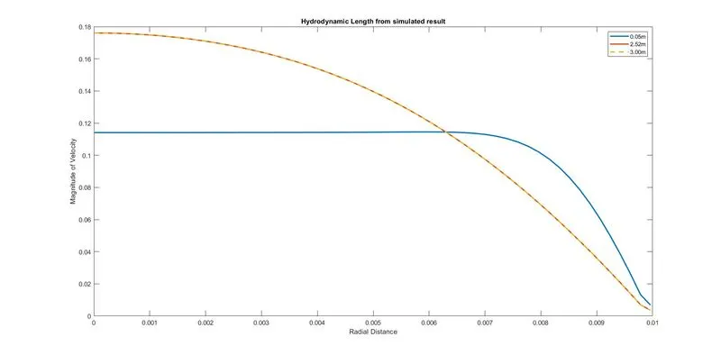
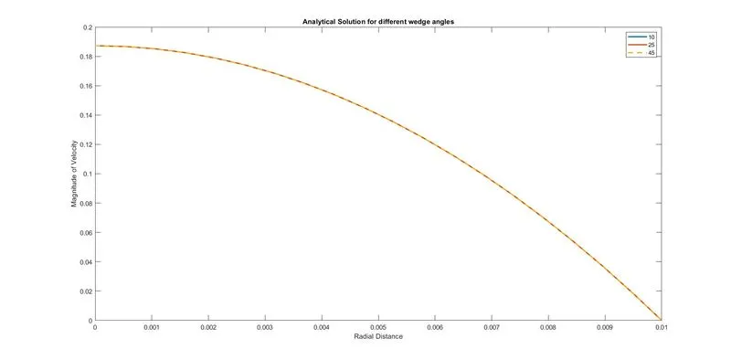
The velocity profile has been plotted for 10deg simulation along with the analytical profile for velocity obtained by solving HP Equations. The numerically calculated velocity profile at 2.52 m and 3 m is clearly identical, which is in accordance with the profile of velocity abtained by solving HP Equation.
2. Fully developed profile.
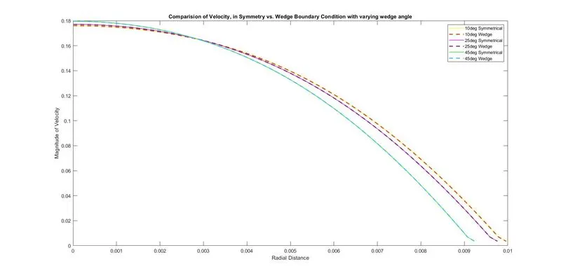
The velocity profile of 10, 25 and 45 deg wedge angle is plotted and compared. Although the numerically calculated values are following the same trend as that of analytically calculated, but the magnitude varies a little. It has been discussed in the comparision section.
3. Maximum Velocity and pressure drop
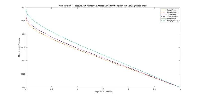
The velocity profile along the cross-section and pressure profile along the length has been plotted. The maximum velocity in the numerical calculations lies around 0.18 m/s which is slightly less when compared with the analytical calculations.
The pressure drop for all the wedge angle was found around 0.02 which is fairly close to the analytical calculations.
4. Shear Stress Calculation
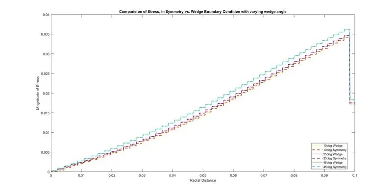
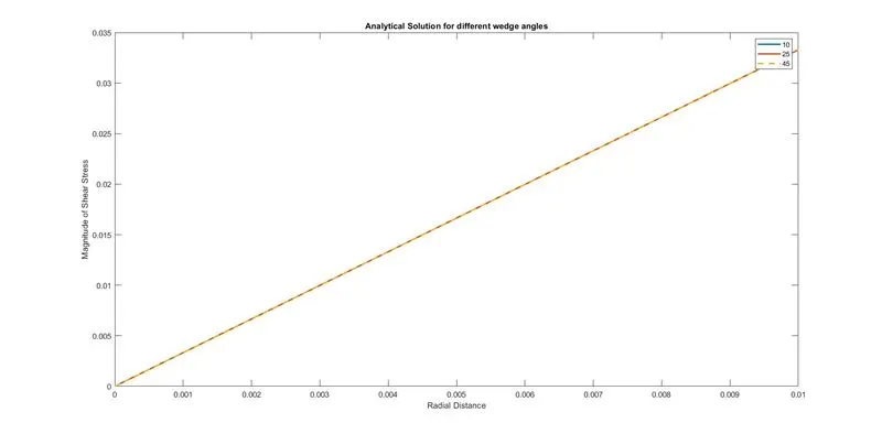
The shear stress has been post processed and plotted for all the wedge angles. The resuls has also been compared with that of the analytical calculation. The maximum Shear stress is found to be similar to that of the analytical calculation.
5. Difference between Wedge and Symmetry boundary conditions.
Since they both are used to define geometries and calculations for axisymmetric calculations, in wedge BC, there is a need of coordinate transformation for the wedge angle whereas in symmetry, its a mirroring over the plane.
Comparing the angle of wedge with the analytical results, The greater the angle is the closer it appears to the analytical results.