Week 12 - Symmetry vs Wedge vs HP equation
Symmetry vs Wedge vs HP equation
Aim:-
- Prefer flow through pipe problem statement from the previous project and solve it using symmetry boundary condition instead of on the wedge.
- Write a Matlab program that takes an angle as input and generates a 'blockMeshDict' file.
- Generate BlockMeshDict program file different symmetry angle of 10o, 25o, and 45o.
- Run created BlockMeshFile in OpenFOAM and compare results with previous analytical results obtained from Hage Poisuelle’s equation and Numerical results with wedge boundary conditions.
- Lastly, write a report explaining all the codes, plots, and figures.
Objectives:-
- write down codes in Matlab to write in the 'blockMeshDict' file. Also, create input in Matlab to run a program to save files for the various angles.
- Open OpenFOAM tutorials and find the solver to solve the incompressible-laminar-viscous flow problem.
- The next step is to copy the required file in solver and paste it into the OpenFOAM run folder so that the official file of OpenFoam remains untouched.
- Replace the blockMeshDict file with the blockMeshDict file created in MatLab
- Find the ‘controlDict’ file to edit the start and end times for the simulation.
- In the initial folder ‘0’ edit the initial parameter for velocity and pressure according to the faces of the given domain.
- Use a 'blockMesh' command to generate mesh and checkMesh to verify it.
- Open the simulation file in ParaView and plot the velocity profile at the fully developed point from the inlet.
- Next, calculate the pressure difference over the length of the file.
- Also, calculate shear stress and plot its graph is a fully developed region.
- Extract all the data from paraFoam to read it in the Matlab program.
- Compare generated data with analytical data obtained from Hagen Poiseuill’s equation and numerical data obtained by using wedge boundary conditions.
- Plot velocity graph of fully developed flow for both numerical with wedge and symmetry boundary condition and analytical method.
- We can also compare the pressure difference plot of the complete length of the pipe by both numerical and analytical methods.
- Write a detailed report explaining all the commands and codes used in the project.
Before starting the project, let us first understand the difference between symmetry and wedge boundary conditions.
Difference Between wedge and symmetry boundary condition
in the last project, we have used the wedge boundary condition, which is used for 2-dimensional axisymmetric cases e.g. a cylinder, the geometry is specified as a wedge of small angle (e.g. < 5o ) and 1 cell thick running along the plane of symmetry, straddling one of the coordinates planes. The axisymmetric wedge planes must be specified as separate patches of wedge type.
On the contrary, symmetry boundary conditions use for any (non-planar) patch which uses the symmetry plane slip condition. Usually, this boundary condition used on objects which are symmetrical or mirror by its various side. As we are using it for axisymmetrical pipe or object we can use any angle we want, and for a bigger angle, we can also discretize it along that angular portion which gives us finer results. This mostly considers 3D simulation conditions.
Now, let us compare the results obtained from symmetrical boundary condition simulation on the same previous problem.
Problem statement
For flow in pipe of diameter D, experimental observations show that for “fully developed” flow, laminar flow occurs when `Re_D` < 2300. Therefore, let us consider Re for flow is 2000. Assume diameter of pipe (D)=0.02m and length (L) = 2.5 m. also consider working fluid as water at temperature 25oC so the values of density (rho)=997kg/`m^3` and Dynamic Viscosity (mu)=8.90X10⁻⁴Pa.sec.
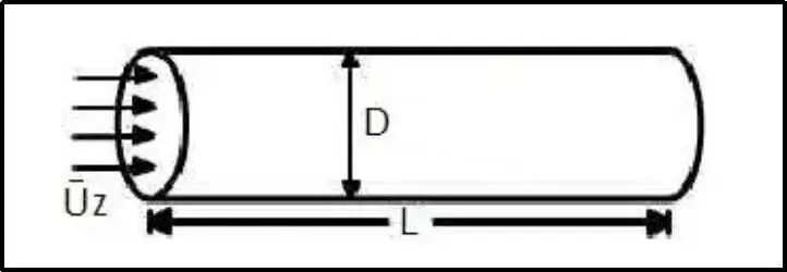
Pre-processing
- For this project, we are going to use the same procedure to simulate our results using symmetry boundary conditions. So, First start terminal in Linux Operating system using ctrl+alt+T buttons on the keyboard or right-click -> Open Terminal.
- Here, exactly as the last project, we have to simulate our problem in OpenFOAM and we are going to solve our problem using tutorials present in OpenFOAM, therefore, just type ‘tut’ to open the OpenFOAM tutorial directory. And type ‘ls’ to identify what kind of tutorials present inside this directory.
- We have to solve incompressible flow simulation for this problem. So select an incompressible directory by typing 'cd incompressible' and then again type 'ls' to explore folders in incompressible folders. And select icoFoam solver which is used for the laminar-viscous flow.
- icoFoam is the solver in OpenFOAM which is used as a transient solver for incompressible, laminar flow of Newtonian fluids.
- (Newtonian fluid is a fluid in which the viscous stress arising from its flow, at every point, are linearly correlated to the local strain rate - the rate of change of its deformation over time. Newtonian fluids are the simplest mathematical models of fluids that account for viscosity.)
- Therefore, we will select the icoFoam folder by typing 'cd icoFoam' and by typing 'ls' we explore this folder in the terminal.
- Here, we have, again to option, cavity and elbow. They both are part of the icoFoam solver and cavity section used to create a required domain and black mesh so select the 'cavity' folder.
- In the cavity, we are, again, going to see the cavity folder, where we have to define our fluid domain and generate block mesh.
- We are going to copy this cavity folder using the 'cp -r cavity' command. Next, rename it as ‘Pipe(45)’, as we did for the ‘Pipe’ folder in our last project, and paste it in OpenFOAM run folder by typing 'cp -r cavity $FOAM_RUN/Pipe(45)'.
- And then open the run folder by typing 'cd $FOAM_RUN'. where we can see the 'Pipe(45)' file.
- Now, we can make any changes to the Pipe file, which will never affect the OpenFOAM official files. Open the Pipe folder. Here, we can provide specifications for our block mesh in the system folder.
- There are four script file system folders and by opening blockMeshDict, we can create a domain and provide the required specification for block mesh.
- Here have to create a blockMeshDict file with Matlab and replace that with the original one. But we already have the program file for wedge boundary condition so we just edit that program for symmetry boundary condition.
File Writing:-
Firstly, for generating mesh along wedge shape cross-section we have to create 8 vertices. It is important for symmetric angel cross-section vertices 0,4 and 3,7 are repeated in an adequate position within the parentheses to indicate that the pare of two vertices that would be occupied this position have been collapsed
fprintf(f1,'vertices\n(\n');
fprintf(f1,'    (0 0 0)\n');
fprintf(f1,('    (%f %f 0)\n'),R*cosd(th/2),R*sind(th/2));
fprintf(f1,('    (%f %f %f)\n'),R*cosd(th/2),R*sind(th/2),L);
fprintf(f1,('    (0 0 %f)\n'),L);
fprintf(f1,'    (0 0 0)\n');
fprintf(f1,('    (%f %f 0)\n'),R*cosd(th/2),-R*sind(th/2));
fprintf(f1,('    (%f %f %f)\n'),R*cosd(th/2),-R*sind(th/2),L);
fprintf(f1,('    (0 0 %f)\n);\n\n'),L);
Next, we are going to define block for meshing, here, we provide vertices number according to order which follow right-hand thumb rule, meaning, the thumb is the z-axis and order of vertices follow rotational order of our other finger.
Then comes, the number of mesh grid that we want to divide along x, y, and z length. We define it as (nx,ny,nz) format in the main program.
Given mesh specification:
- Number of cells along the z-direction(longer dimension) = 500
- Number of cells along with the longer x-direction = 20
- Number of the cell for y-direction =theta/5 (vary according to theta angle)
Lastly, we give simple grading which is cell expansion ratios.
fprintf(f1,'blocks\n(\n');
fprintf(f1,('hex (1 5 6 2 0 4 7 3) (%d %d %d) simpleGrading (1 1 10)\n);\n\n'),nx,ny,nz);
In this case, for edge 5-1 and 6-2, we have a radius curve so we will define this in the edges section following way.
fprintf(f1,'edges\n(\n');
fprintf(f1,'    arc 1 5 (%f 0 0)\n',R);
fprintf(f1,'    arc 6 2 (%f 0 %f)\n);\n\n',R,L);
Next, define the boundary of the problem, in this, we have to define the faces of our 3D block this should be in order according to the right-hand thumb rule. So set faces for this problem following way.
In the patches definition, the same vertices 0,4 and 3,7 are joined creating an empty patch forming the axis of the pipe. the patch type symmetry is used in two faces to indicate that symmetry exists with respect to those two faces and there are no physical walls.
fprintf(f1,'boundary\n(\n');
fprintf(f1,'     inlet\n');
fprintf(f1,'     {\n');
fprintf(f1,'           type patch;\n');
fprintf(f1,'           faces\n');
fprintf(f1,'           (\n');
fprintf(f1,'               (1 0 4 5)\n');
fprintf(f1,'           );\n');
fprintf(f1,'     }\n');
fprintf(f1,'     outlet\n');
fprintf(f1,'     {\n');
fprintf(f1,'           type patch;\n');
fprintf(f1,'           faces\n');
fprintf(f1,'           (\n');
fprintf(f1,'               (2 6 7 3)\n');
fprintf(f1,'           );\n');
fprintf(f1,'     }\n');
fprintf(f1,'     front\n');
fprintf(f1,'     {\n');
fprintf(f1,'           type symmetry;\n');
fprintf(f1,'           faces\n');
fprintf(f1,'           (\n');
fprintf(f1,'               (1 2 3 0)\n');
fprintf(f1,'           );\n');
fprintf(f1,'     }\n');
fprintf(f1,'     back\n');
fprintf(f1,'     {\n');
fprintf(f1,'           type symmetry;\n');
fprintf(f1,'           faces \n');
fprintf(f1,'           (\n');
fprintf(f1,'               (7 6 5 4)\n');
fprintf(f1,'           );\n');
fprintf(f1,'     }\n');
fprintf(f1,'     pipewall\n');
fprintf(f1,'     {\n');
fprintf(f1,'           type wall;\n');
fprintf(f1,'           faces\n');
fprintf(f1,'           (\n');
fprintf(f1,'               (1 5 6 2)\n');
fprintf(f1,'           );\n');
fprintf(f1,'     }\n');
fprintf(f1,'     axis\n');
fprintf(f1,'     {\n');
fprintf(f1,'           type empty;\n');
fprintf(f1,'           faces\n');
fprintf(f1,'           (\n');
fprintf(f1,'               (0 3 7 4)\n');
fprintf(f1,'           );\n');
fprintf(f1,'      }\n');
fprintf(f1,');\n\n');
fprintf(f1,'mergePatchPairs\n');
fprintf(f1,'(\n');
fprintf(f1,');\n\n');
fprintf(f1,'// ************************************************************************* // \n');
Running Matlab codes after making previous changes we will get the following blockMeshDict codes.
/*--------------------------------*- C++ -*----------------------------------*\
  =========                 |
  \\      /  F ield         | OpenFOAM: The Open Source CFD Toolbox
   \\    /   O peration     | Website:  https://openfoam.org
    \\  /    A nd           | Version:  8
     \\/     M anipulation  |
\*---------------------------------------------------------------------------*/
FoamFile
{
    version     2.0;
    format      ascii;
    class       dictionary;
    object      blockMeshDict;
}
// * * * * * * * * * * * * * * * * * * * * * * * * * * * * * * * * * * * * * //

convertToMeters 1;

vertices
(
    (0 0 0)
    (0.009239 0.003827 0)
    (0.009239 0.003827 2.500000)
    (0 0 2.500000)
    (0 0 0)
    (0.009239 -0.003827 0)
    (0.009239 -0.003827 2.500000)
    (0 0 2.500000)
);

blocks
(
hex (1 5 6 2 0 4 7 3) (9 500 20) simpleGrading (1 1 10)
);

edges
(
    arc 1 5 (0.010000 0 0)
    arc 6 2 (0.010000 0 2.500000)
);

boundary
(
     inlet
     {
           type patch;
           faces
           (
               (1 0 4 5)
           );
     }
     outlet
     {
           type patch;
           faces
           (
               (2 6 7 3)
           );
     }
     front
     {
           type symmetry;
           faces
           (
               (1 2 3 0)
           );
     }
     back
     {
           type symmetry;
           faces
           (
               (7 6 5 4)
           );
     }
     pipewall
     {
           type wall;
           faces
           (
               (1 5 6 2)
           );
     }
     axis
     {
           type empty;
           faces
           (
               (0 3 7 4)
           );
      }
);

mergePatchPairs
(
);

// ************************************************************************* //
Copy blockMeshDict file and replace it in the system directory of the Pipe(45) folder and by running this block mesh file we will get the following mesh:
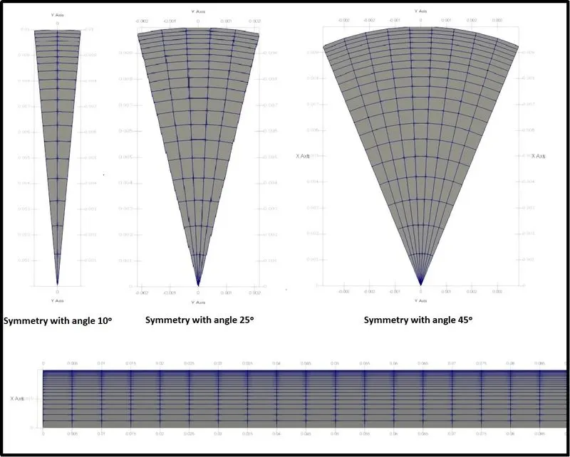
Furthermore, we are editing the ‘controlDict’ file to provide time limits - start time and end time. Also to represent `deltat`. While the selection of `deltat` CFL value should be less than 1. otherwise, the solution could be stopped forcibly or it may diverge at the time of converging. So make the following changes in the ‘controlDict’ file.
Boundary and initial conditions
Then, we have to define the initial value for pressure and velocity. In order to do that, we have to go back to Pipe(45) directory using the ‘cd ..’ command and select a folder named ‘0’, which stands for initial values. In this case initial value for pressure and velocity.
When solving circulating internal flow, the most common boundary conditions are to fix an inlet velocity and an outlet pressure.
And for symmetry boundary condition just define to side faces to symmetry.
Initial setting for pressure
/*--------------------------------*- C++ -*----------------------------------*\
  =========                 |
  \\      /  F ield         | OpenFOAM: The Open Source CFD Toolbox
   \\    /   O peration     | Website:  https://openfoam.org
    \\  /    A nd           | Version:  8
     \\/     M anipulation  |
\*---------------------------------------------------------------------------*/
FoamFile
{
    version     2.0;
    format      ascii;
    class       volScalarField;
    object      p;
}
// * * * * * * * * * * * * * * * * * * * * * * * * * * * * * * * * * * * * * //

dimensions      [0 2 -2 0 0 0 0];

internalField   uniform 0;

boundaryField
{
    inlet
    {
        type            zeroGradient;
    }

    outlet
    {
        type            fixedValue;
        value           uniform 0;
    }

    front
    {
        type            symmetry;
    }

    back
    {
        type            symmetry;
    }

    axis
    {
        type            empty;
    }

    pipewall
    {
        type            zeroGradient;
    }
}

// ************************************************************************* //
In the U dictionary, one can find out a new type of boundary condition: inlet and outlet. It switches U and p between fixed value and zero gradients: the first when the flow is in-going and the second when it is outgoing.
For example: in a circular pipe case, the outlet velocity will always be adapted to the conditions according to zero gradients except if there is an inflow at the outlet patch. If this happens, to this inflow velocity it is assigned the value specified under the inlet-outlet instruction and so the flow will always be outgoing.
Lastly, define side faces to symmetry instead of wedge boundary condition.
Initial setting for Velocity
/*--------------------------------*- C++ -*----------------------------------*\
  =========                 |
  \\      /  F ield         | OpenFOAM: The Open Source CFD Toolbox
   \\    /   O peration     | Website:  https://openfoam.org
    \\  /    A nd           | Version:  8
     \\/     M anipulation  |
\*---------------------------------------------------------------------------*/
FoamFile
{
    version     2.0;
    format      ascii;
    class       volVectorField;
    object      U;
}
// * * * * * * * * * * * * * * * * * * * * * * * * * * * * * * * * * * * * * //

dimensions      [0 1 -1 0 0 0 0];

internalField   uniform (0 0 0);

boundaryField
{
    inlet
    {
        type            fixedValue;
        value           uniform (0 0 0.09373);
    }

    outlet
    {
        type            zeroGradient;
    }

    front
    {
        type            symmetry;
    }

    back
    {
        type            symmetry;
    }

    axis
    {
        type            empty;
    }

    pipewall
    {
        type            noSlip;
    }
}

// ************************************************************************* //
Next, we are going to keep the same dynamic viscosity as we kept in the previous project of wedge boundary condition.
/*--------------------------------*- C++ -*----------------------------------*\
  =========                 |
  \\      /  F ield         | OpenFOAM: The Open Source CFD Toolbox
   \\    /   O peration     | Website:  https://openfoam.org
    \\  /    A nd           | Version:  8
     \\/     M anipulation  |
\*---------------------------------------------------------------------------*/
FoamFile
{
    version     2.0;
    format      ascii;
    class       dictionary;
    location    "constant";
    object      transportProperties;
}
// * * * * * * * * * * * * * * * * * * * * * * * * * * * * * * * * * * * * * //

nu              [0 2 -1 0 0 0 0] 8.90e-4;


// ************************************************************************* //
After deploying mesh, now we are ready to run the simulation. Like last time, this time also we are running the simulation for viscus-laminar flow that's why we will choose our solver as icoFoam. Hence, just type ‘icoFoam’ and simulation will start.
Post-processing
Now, let us view the results in ParaView by using the ‘paraFoam’ command.
RESULTS OF THE SIMULATION
Velocity at various distances from the inlet of pipe and comparison of it with fully developed velocity flow at distance 2.32 from the inlet of the pipe:-
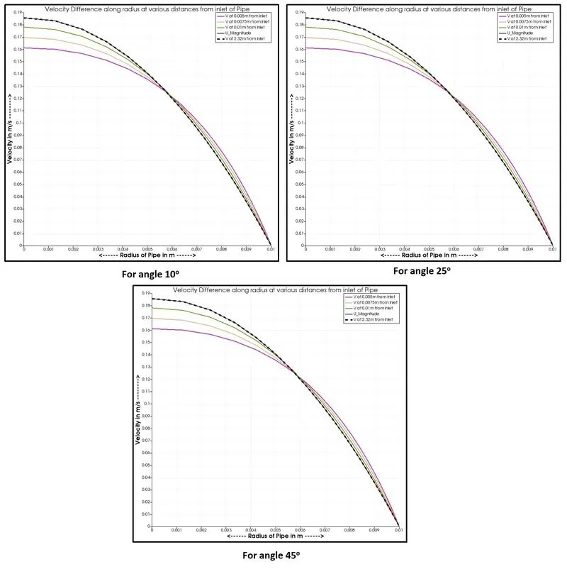
If we notice all three conditions of angles in symmetry boundary conditions, the overall results are pretty much identical to each other.
As we can see above graphs, portrays the velocity profile along radius at various distances from the inlet. So we can observe that as water moving forward through pipe its velocity profile along the radius of the pipe is stabilizing and there is a point within a length of the point where it does not change that point is called fully developed flow region. And it comes after entrance length which we calculated in the above section of this project.
Pressure change along the length of pipe:-
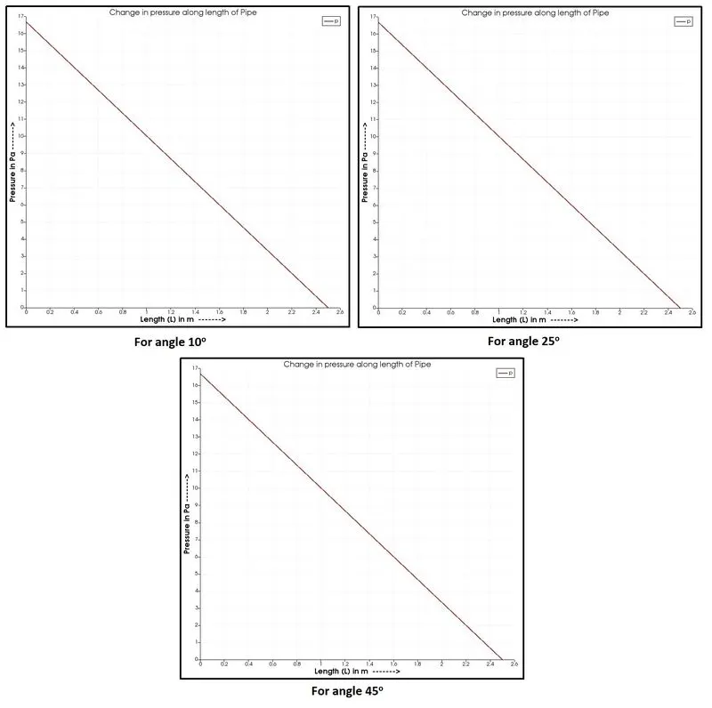
We can notice the same thing with pressure, results for pressure for all three cases are very similar to each other. If we check the pressure plots, the pressure gradually decreasing along the length of the pipe as the velocity increases.
Shear stress along the radius at the developed region of the pipe:-
We saw our velocity results with symmetry boundary conditions for different angles, which are the same for all three cases, therefore, we can say that their shear stress results will be also identical to each other. And this can be validated after plotting shear stress results.
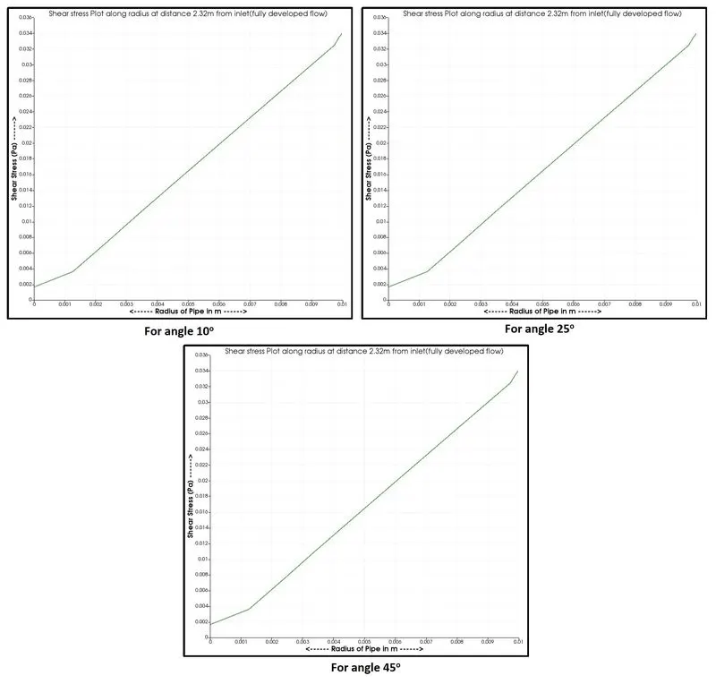
If we focus on shear stress along the radius of the pipe, in a fully developed flow region, we can observe there is very little shear stress at the center as there is no wall is present to restrict the flow of fluid. But from the center to the wall, we can see, the shear stress increasing gradually and its value near the wall is maximum.
In our next step, we will extract all the data from ParaView by saving spreadsheets in .csv format to read it in Matlab.
File Reading
For file reading, we are going to make a separate function program for each method as we did in our last project. We have to read the following file in this project.
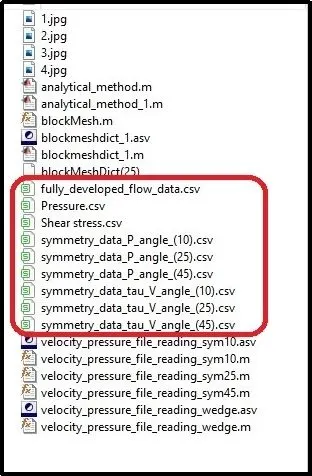
In order to keep the program simpler, we are going to create 4 different functions for 4 different cases to read the file. One for wedge boundary condition, Second for symmetry boundary condition for 10o angle, Third for symmetry boundary condition for 25o angle and Fourth also for symmetry boundary condition but for 45o angle.
for instance, if we have to read a file of symmetry boundary condition for a 10o angle, start reading a file using the following command.
%% Reading Velocity File Extracted from paraView
f2 = fopen('symmetry_data_tau_V_angle_(10).csv','r');
We can use 'fgetl' to read lines or skip lines sequence wise. So, by typing 'fgetl' we will skip the first line and then create a loop to read file line by line and store velocity and length data in V_sym10_n and L_sym10_n.
Lastly, we use str2double to convert string data to number data.
A=fgetl(f2);
for i = 1:1000
    C = fgetl(f2);
    D = strsplit(C,',');
    V_sym10_n(i) = D(7);
    L_sym10_n(i) = D(13);
end
V_sym10_n=str2double(V_sym10_n');
L_sym10_n=str2double(L_sym10_n');
Similar way, we will read and store pressure and shear stress data in Matlab function.
%% Reading Pressure File Extracted from paraView
f3 = fopen('symmetry_data_P_angle_(10).csv','r');
A=fgetl(f3);
for i = 1:1000
    C = fgetl(f3);
    D = strsplit(C,',');
    P_sym10_n(i) = D(4);
    L_sym10_nn(i) = D(6);
end
P_sym10_n=str2double(P_sym10_n');
L_sym10_nn=str2double(L_sym10_nn');


%% Reading Shear Stress File Extracted from paraView
f4 = fopen('symmetry_data_tau_V_angle_(10).csv','r');
A=fgetl(f4);
for i = 1:1000
    C = fgetl(f4);
    D = strsplit(C,',');
    tau_sym10_n(i) = D(9);
end
tau_sym10_n=-(str2double(tau_sym10_n'));
Here, we are going to compare data obtained from symmetry boundary conditions with analytical data and numerical data by wedge boundary conditions which we calculated in our last project.
Hence, let us call the function which stores our Numerical results and plot the data.
Velocity comparison Symmetry vs Wedge vs HP equation(analytical results)
%% [1]-Plotting - Velocity comparison from analytical method and numerical method
figure(1)
set(gcf, 'Position',  [100, 100, 800, 800])
plot(r,Vr,'m','linewidth',1)
hold on
plot(L_wedge_n,V_wedge_n,'--','color','k','linewidth',2.5)
plot(L_sym10_n,V_sym10_n,'color','y','linewidth',2.5)
plot(L_sym25_n,V_sym25_n,'--','color','r','linewidth',2)
plot(L_sym45_n,V_sym45_n,':','color','b','linewidth',1)
xlabel('<---- Radius of pipe in m ---->','fontweight','bold','fontsize',14)
ylabel(' Velocity in m/s ------>','fontweight','bold','fontsize',14)
title('Velocity variation over the radius of pipe','fontsize',18)
legend('Analytical method','Numerical method by wedge Boundary Condition','Numerical method by symmetry BC with 10^o angle','Numerical method by symmetry BC with 25^o angle','Numerical method by symmetry BC with 45^o angle')
grid on
Result Plot:-
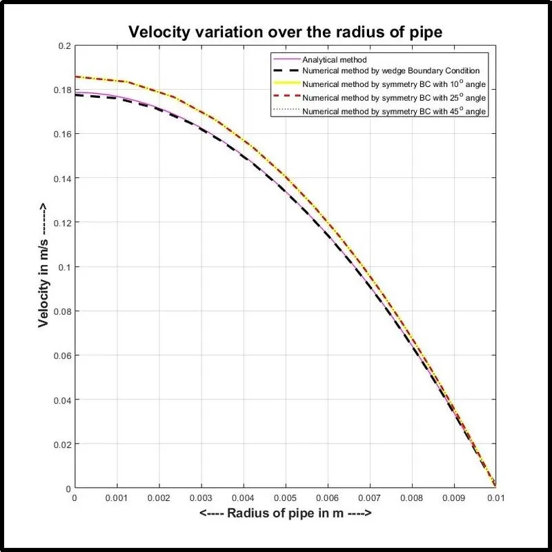
The above line graph exhibits information about velocity variation with the Exact or analytical method, the numerical method by wedge Boundary condition, Numerical analytical method by symmetry boundary condition with 10o, 25o, and 40o respectively along the radius of the pipe.
Glimpse over a graph portrays some intriguing pattern in which numerical results with wedge boundary conditions showing less error than numerical results with symmetry boundary conditions. If we talk about symmetry boundary conditions, we can notice, results are independent of the angle we select to simulate pipe flow. But as symmetric boundary condition use for symmetrical or mirror type object we can see its showing lot deviation near the center of the pipe. To check those errors in the exact number lest run the following codes.
Max Error
%Max Velocity Error
Error_max_wedge_bc = max(max(abs(Vr-V_wedge_n)))
Error_max_symmetry10_bc = max(max(abs(Vr-V_sym10_n)))
Error_max_symmetry25_bc = max(max(abs(Vr-V_sym25_n)))
Error_max_symmetry45_bc = max(max(abs(Vr-V_sym45_n)))
In order to get an error, in the above codes, we are subtracting all numerical velocity results from exact results so we can get differences and then we are extracting absolute maximum error from all deviations.
Output Result:-
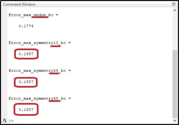
After running the aforementioned line of codes we will get the above results and we can clearly see the simulation method with symmetry boundary condition showing more error than wedge boundary condition. We can also notice, we are getting the same error results for each angle so we can utterly say that in the pipe case we can select any angle for the simulation as results independent with respect to angle.
Velocity variation over the Diameter of pipe at the developed region for various method
%% [4]-Plotting - Velocity comparison from analytical method and numerical method
figure(4)
set(gcf, 'Position',  [100, 100, 1200, 800])
plot(Vr,r,'m',Vr,-r,'m','linewidth',1)
hold on
plot(V_wedge_n,L_wedge_n,'--',V_wedge_n,-L_wedge_n,'--','color','k','linewidth',2.5,'DisplayName','Numerical method by wedge Boundary Condition')
plot(V_sym10_n,L_sym10_n,'y',V_sym10_n,-L_sym10_n,'y','linewidth',2.5)
plot(V_sym25_n,L_sym25_n,'--',V_sym25_n,-L_sym25_n,'--','color','r','linewidth',2)
plot(V_sym45_n,L_sym45_n,':',V_sym45_n,-L_sym45_n,':','color','b','linewidth',1)
ylabel('<---- Diameter of pipe in m ---->','fontweight','bold','fontsize',14)
xlabel(' Velocity in m/s ------>','fontweight','bold','fontsize',14)
title('Velocity variation over the Diameter of pipe','fontsize',18)
grid on
Result Plot:-
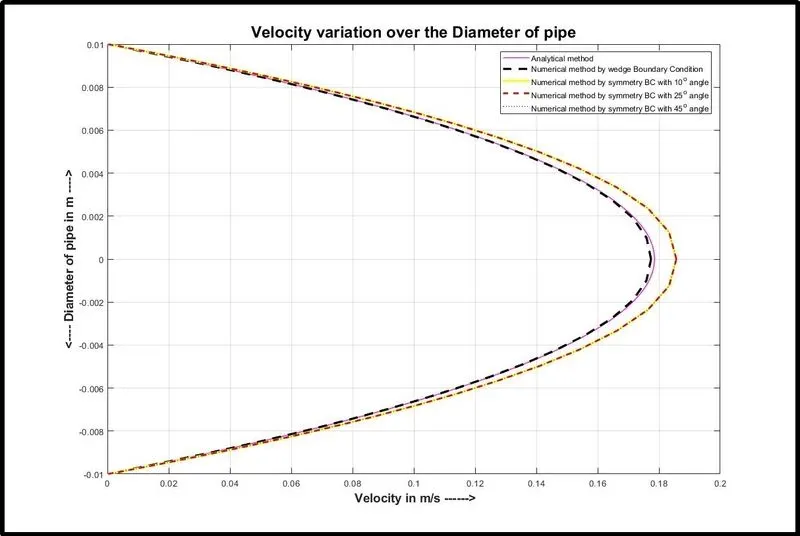
The above figure depicts the exact plot of velocity distribution over complete diameter at a fully developed region. These are the same results as we saw in the velocity distribution figure before. Therefore, it's just to visualize overall flow distribution in a fully developed area. Next, we are going to see pressure distribution over a length of pipe.
Pressure comparison Symmetry vs Wedge vs HP equation(analytical results)
%% [2]-Plotting - Pressure comparison from analytical method and numerical method
figure(2)
set(gcf, 'Position',  [100, 100, 800, 800])
plot(L_an,P_drop,'m','linewidth',1)
hold on
plot(L_wedge_nn,P_wedge_n,'--','color','k','linewidth',2.5)
plot(L_sym10_nn,P_sym10_n,'color','y','linewidth',2.5)
plot(L_sym25_nn,P_sym25_n,'--','color','r','linewidth',2)
plot(L_sym45_nn,P_sym45_n,':','color','b','linewidth',1)
xlabel('<---- Length of pipe in m ---->','fontweight','bold','fontsize',14)
ylabel(' Pressure in Pa ------>','fontweight','bold','fontsize',14)
title('Pressure variation over the length of pipe','fontsize',18)
legend('Analytical method','Numerical method by wedge Boundary Condition','Numerical method by symmetry BC with 10^o angle','Numerical method by symmetry BC with 25^o angle','Numerical method by symmetry BC with 45^o angle')
grid on
Result Plot:-
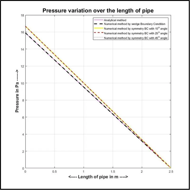
In the pressure distribution line graph, we can notice numerical results with wedge boundary conditions are perfectly matching with analytical results but the output from symmetry boundary condition showing error. At the stating point of the pipe, it showing pressure little higher than the analytical results. And, here also, we can notice, the results are not affected by the angles of the domain region of the pipe.
Shear stress comparison Symmetry vs Wedge vs HP equation(analytical results)
%% [3]-Plotting - Pressure comparison from analytical method and numerical method
figure(3)
set(gcf, 'Position',  [100, 100, 800, 800])
plot(L_wedge_n,tau_wedge_n,'color','g','linewidth',2)
hold on
plot(L_sym10_n,tau_sym10_n,'color','y','linewidth',2.5)
plot(L_sym25_n,tau_sym25_n,'--','color','r','linewidth',2)
plot(L_sym45_n,tau_sym45_n,':','color','b','linewidth',1)
xlabel('<---- Radius of pipe in m ---->','fontweight','bold','fontsize',14)
ylabel('Shear Stress Pa ------>','fontweight','bold','fontsize',14)
title('Shear Stress variation over the radius of pipe','fontsize',18)
legend({'Numerical method by wedge Boundary Condition','Numerical method by symmetry BC with 10^o angle','Numerical method by symmetry BC with 25^o angle','Numerical method by symmetry BC with 45^o angle'},'location','northwest')
grid on
Result Plot:-
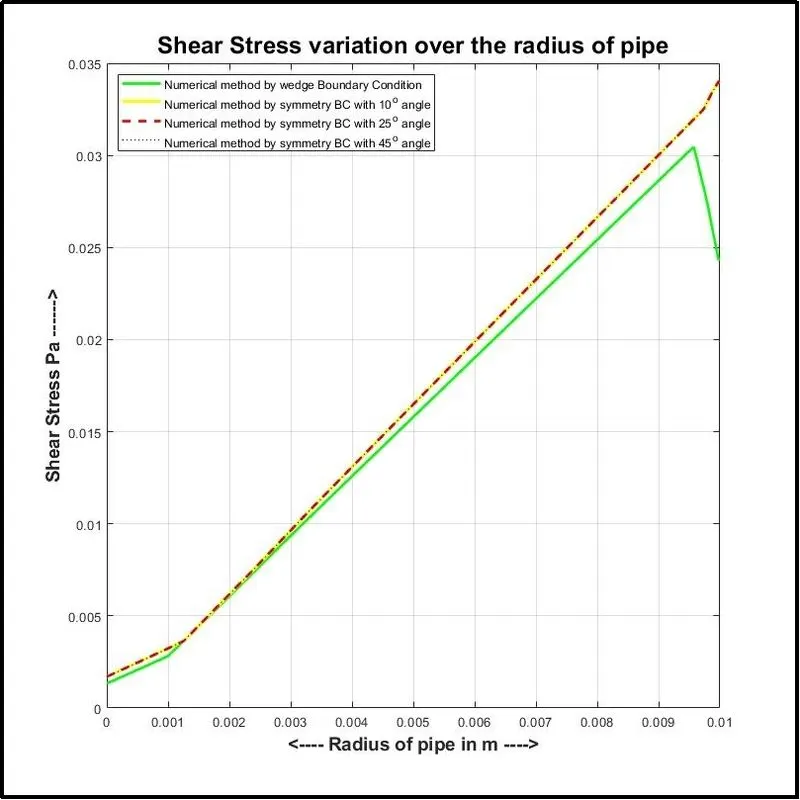
Lastly, if we talk about shear stress, as there is the difference in results of velocity so there will be variations in shear stress also, as we can see, shear stresses in symmetry boundary condition simulation are shown little difference compare to wedge boundary conditions.
Conclusion:-
- We are able to calculate our results for a pipe using symmetry boundary conditions with angle 10o, 25o, and 45o in OpenFOAM.
- In symmetrical boundary conditions, as the angle of the pipe increases the number of grids also must have to increase. Which led to an increase in the count number of finite volumes within the domain. Therefore, calculation time also increases. And this is the reason we need more time to simulate domain with angle 45o than the other two given angles of the domain.
- As we are getting the same results with every angle we selected for the simulation, it will be a good choice to select minimum angel for simulation which save our large simulation time to get the required results
- Lastly, wedge boundary conditions are most suitable for the simulation of axisymmetric 2D objects and symmetry use for symmetrical and mirror 2D or 3D objects. Hence, for pipe simulation, wedge boundary conditions are more preferable as they showing less error than the symmetrical boundary condition.
Reference:-
[1] Previous Project-Week 11 - Simulation of Flow through a pipe in OpenFoam : Skill-Lync (skill-lync.com)
Complete Function Program for BlockMeshDict File (File Writing)
function[f1] = blockMesh(R,th,L,nx,ny,nz)

%% Writing BlockMeshDict file for openFoam
f1 = fopen('blockMeshDict(25)','w');

fprintf(f1,"/*--------------------------------*- C++ -*----------------------------------*\\ \n");
fprintf(f1,'  =========                 | \n');
fprintf(f1,'  \\\\      /  F ield         | OpenFOAM: The Open Source CFD Toolbox \n');
fprintf(f1,'   \\\\    /   O peration     | Website:  https://openfoam.org \n');
fprintf(f1,'    \\\\  /    A nd           | Version:  8 \n');
fprintf(f1,'     \\\\/     M anipulation  |\n');
fprintf(f1,"\\*---------------------------------------------------------------------------*/ \n");
fprintf(f1,'FoamFile \n');
fprintf(f1,'{ \n');
fprintf(f1,'    version     2.0;\n');
fprintf(f1,'    format      ascii;\n');
fprintf(f1,'    class       dictionary;\n');
fprintf(f1,'    object      blockMeshDict;\n');
fprintf(f1,'} \n');
fprintf(f1,'// * * * * * * * * * * * * * * * * * * * * * * * * * * * * * * * * * * * * * // \n\n');
fprintf(f1,'convertToMeters 1; \n\n');
fprintf(f1,'vertices\n(\n');
fprintf(f1,'    (0 0 0)\n');
fprintf(f1,('    (%f %f 0)\n'),R*cosd(th/2),R*sind(th/2));
fprintf(f1,('    (%f %f %f)\n'),R*cosd(th/2),R*sind(th/2),L);
fprintf(f1,('    (0 0 %f)\n'),L);
fprintf(f1,'    (0 0 0)\n');
fprintf(f1,('    (%f %f 0)\n'),R*cosd(th/2),-R*sind(th/2));
fprintf(f1,('    (%f %f %f)\n'),R*cosd(th/2),-R*sind(th/2),L);
fprintf(f1,('    (0 0 %f)\n);\n\n'),L);
fprintf(f1,'blocks\n(\n');
fprintf(f1,('hex (1 5 6 2 0 4 7 3) (%d %d %d) simpleGrading (1 1 10)\n);\n\n'),nx,ny,nz);
fprintf(f1,'edges\n(\n');
fprintf(f1,'    arc 1 5 (%f 0 0)\n',R);
fprintf(f1,'    arc 6 2 (%f 0 %f)\n);\n\n',R,L);
fprintf(f1,'boundary\n(\n');
fprintf(f1,'     inlet\n');
fprintf(f1,'     {\n');
fprintf(f1,'           type patch;\n');
fprintf(f1,'           faces\n');
fprintf(f1,'           (\n');
fprintf(f1,'               (1 0 4 5)\n');
fprintf(f1,'           );\n');
fprintf(f1,'     }\n');
fprintf(f1,'     outlet\n');
fprintf(f1,'     {\n');
fprintf(f1,'           type patch;\n');
fprintf(f1,'           faces\n');
fprintf(f1,'           (\n');
fprintf(f1,'               (2 6 7 3)\n');
fprintf(f1,'           );\n');
fprintf(f1,'     }\n');
fprintf(f1,'     front\n');
fprintf(f1,'     {\n');
fprintf(f1,'           type symmetry;\n');
fprintf(f1,'           faces\n');
fprintf(f1,'           (\n');
fprintf(f1,'               (1 2 3 0)\n');
fprintf(f1,'           );\n');
fprintf(f1,'     }\n');
fprintf(f1,'     back\n');
fprintf(f1,'     {\n');
fprintf(f1,'           type symmetry;\n');
fprintf(f1,'           faces \n');
fprintf(f1,'           (\n');
fprintf(f1,'               (7 6 5 4)\n');
fprintf(f1,'           );\n');
fprintf(f1,'     }\n');
fprintf(f1,'     pipewall\n');
fprintf(f1,'     {\n');
fprintf(f1,'           type wall;\n');
fprintf(f1,'           faces\n');
fprintf(f1,'           (\n');
fprintf(f1,'               (1 5 6 2)\n');
fprintf(f1,'           );\n');
fprintf(f1,'     }\n');
fprintf(f1,'     axis\n');
fprintf(f1,'     {\n');
fprintf(f1,'           type empty;\n');
fprintf(f1,'           faces\n');
fprintf(f1,'           (\n');
fprintf(f1,'               (0 3 7 4)\n');
fprintf(f1,'           );\n');
fprintf(f1,'      }\n');
fprintf(f1,');\n\n');
fprintf(f1,'mergePatchPairs\n');
fprintf(f1,'(\n');
fprintf(f1,');\n\n');
fprintf(f1,'// ************************************************************************* // \n');
fclose(f1);


end
Complete Function Program for Symmetry Boundary condition for angle 10o (File Reading)
function [L_sym10_n,V_sym10_n,L_sym10_nn,P_sym10_n,tau_sym10_n] = velocity_pressure_file_reading_sym10()


%% Reading Velocity File Extracted from paraView
f2 = fopen('symmetry_data_tau_V_angle_(10).csv','r');
A=fgetl(f2);
for i = 1:1000
    C = fgetl(f2);
    D = strsplit(C,',');
    V_sym10_n(i) = D(7);
    L_sym10_n(i) = D(13);
end
V_sym10_n=str2double(V_sym10_n');
L_sym10_n=str2double(L_sym10_n');


%% Reading Pressure File Extracted from paraView
f3 = fopen('symmetry_data_P_angle_(10).csv','r');
A=fgetl(f3);
for i = 1:1000
    C = fgetl(f3);
    D = strsplit(C,',');
    P_sym10_n(i) = D(4);
    L_sym10_nn(i) = D(6);
end
P_sym10_n=str2double(P_sym10_n');
L_sym10_nn=str2double(L_sym10_nn');


%% Reading Shear Stress File Extracted from paraView
f4 = fopen('symmetry_data_tau_V_angle_(10).csv','r');
A=fgetl(f4);
for i = 1:1000
    C = fgetl(f4);
    D = strsplit(C,',');
    tau_sym10_n(i) = D(9);
end
tau_sym10_n=(str2double(tau_sym10_n'));

end
Complete Function Program for Symmetry Boundary condition for angle 25o (File Reading)
function [L_sym25_n,V_sym25_n,L_sym25_nn,P_sym25_n,tau_sym25_n] = velocity_pressure_file_reading_sym25()


%% Reading Velocity File Extracted from paraView
f2 = fopen('symmetry_data_tau_V_angle_(10).csv','r');
A=fgetl(f2);
for i = 1:1000
    C = fgetl(f2);
    D = strsplit(C,',');
    V_sym25_n(i) = D(7);
    L_sym25_n(i) = D(13);
end
V_sym25_n=str2double(V_sym25_n');
L_sym25_n=str2double(L_sym25_n');


%% Reading Pressure File Extracted from paraView
f3 = fopen('symmetry_data_P_angle_(10).csv','r');
A=fgetl(f3);
for i = 1:1000
    C = fgetl(f3);
    D = strsplit(C,',');
    P_sym25_n(i) = D(4);
    L_sym25_nn(i) = D(6);
end
P_sym25_n=str2double(P_sym25_n');
L_sym25_nn=str2double(L_sym25_nn');


%% Reading Shear Stress File Extracted from paraView
f4 = fopen('symmetry_data_tau_V_angle_(10).csv','r');
A=fgetl(f4);
for i = 1:1000
    C = fgetl(f4);
    D = strsplit(C,',');
    tau_sym25_n(i) = D(9);
end
tau_sym25_n=(str2double(tau_sym25_n'));

end
Complete Function Program for Symmetry Boundary condition for angle 45o (File Reading)
function [L_sym45_n,V_sym45_n,L_sym45_nn,P_sym45_n,tau_sym45_n] = velocity_pressure_file_reading_sym45()


%% Reading Velocity File Extracted from paraView
f2 = fopen('symmetry_data_tau_V_angle_(10).csv','r');
A=fgetl(f2);
for i = 1:1000
    C = fgetl(f2);
    D = strsplit(C,',');
    V_sym45_n(i) = D(7);
    L_sym45_n(i) = D(13);
end
V_sym45_n=str2double(V_sym45_n');
L_sym45_n=str2double(L_sym45_n');


%% Reading Pressure File Extracted from paraView
f3 = fopen('symmetry_data_P_angle_(10).csv','r');
A=fgetl(f3);
for i = 1:1000
    C = fgetl(f3);
    D = strsplit(C,',');
    P_sym45_n(i) = D(4);
    L_sym45_nn(i) = D(6);
end
P_sym45_n=str2double(P_sym45_n');
L_sym45_nn=str2double(L_sym45_nn');


%% Reading Shear Stress File Extracted from paraView
f4 = fopen('symmetry_data_tau_V_angle_(10).csv','r');
A=fgetl(f4);
for i = 1:1000
    C = fgetl(f4);
    D = strsplit(C,',');
    tau_sym45_n(i) = D(9);
end
tau_sym45_n=(str2double(tau_sym45_n'));


end
Complete Main Program with input for angle
clear all
close all
clc

%% Input parameters
% Reynold's Number
Re = 2000;
% Total Length of pipe(m)
L = 2.5;
% Diameter of pipe in meters
D = 0.02;
% Wedge Angle in degrees
th = input('<0> Wedge Angle in degrees - ');
% Density (kg/m^3)
rho = 997;
% Dynamic Viscosity (Pa.sec)
mu = 8.90e-4;
% Radius of pipe(m)
R = D/2;


% Entrance Length
Le = 0.058*Re*D;

% Number of cells in x,y,z Directions
nx = round(th/5);
ny = 500;
nz = 20;

%% BlockMeshDict file writting
[f1] = blockMesh(R,th,L,nx,ny,nz);


%% Calculations for Analytical methods
%% Velocity
% Analytical results
% Average Velcity
V_avg = (Re*mu)/(rho*D)

% Velocity at every radius in a fully developed region
r = linspace(0,R,1000);
Vr=2*V_avg*(1-(r.^2/R^2));
% Velocity at center
V_max = 2*V_avg


%% Pressure Drop
% Pressure Drop in across the length of pipe
L_an = linspace(0,L,1000);
P_drop = (32*mu.*L_an.*V_avg)/D^2;
P_drop = fliplr(P_drop);


%% Wall Shear Stress
% Darcy Friction Factor
f = 64/Re;
% wall Shear stress
tau_w = (f/4)*((rho*V_avg^2)/2);


%% Velocity and Pressure file reading
[L_wedge_n,V_wedge_n,L_wedge_nn,P_wedge_n,tau_wedge_n] =velocity_pressure_file_reading_wedge();
[L_sym10_n,V_sym10_n,L_sym10_nn,P_sym10_n,tau_sym10_n] = velocity_pressure_file_reading_sym10();
[L_sym25_n,V_sym25_n,L_sym25_nn,P_sym25_n,tau_sym25_n] = velocity_pressure_file_reading_sym25();
[L_sym45_n,V_sym45_n,L_sym45_nn,P_sym45_n,tau_sym45_n] = velocity_pressure_file_reading_sym45();

%% [1]-Plotting - Velocity comparison from analytical method and numerical method
figure(1)
set(gcf, 'Position',  [100, 100, 800, 800])
plot(r,Vr,'m','linewidth',1)
hold on
plot(L_wedge_n,V_wedge_n,'--','color','k','linewidth',2.5)
plot(L_sym10_n,V_sym10_n,'color','y','linewidth',2.5)
plot(L_sym25_n,V_sym25_n,'--','color','r','linewidth',2)
plot(L_sym45_n,V_sym45_n,':','color','b','linewidth',1)
xlabel('<---- Radius of pipe in m ---->','fontweight','bold','fontsize',14)
ylabel(' Velocity in m/s ------>','fontweight','bold','fontsize',14)
title('Velocity variation over the radius of pipe','fontsize',18)
legend('Analytical method','Numerical method by wedge Boundary Condition','Numerical method by symmetry BC with 10^o angle','Numerical method by symmetry BC with 25^o angle','Numerical method by symmetry BC with 45^o angle')
grid on


%% [2]-Plotting - Pressure comparison from analytical method and numerical method
figure(2)
set(gcf, 'Position',  [100, 100, 800, 800])
plot(L_an,P_drop,'m','linewidth',1)
hold on
plot(L_wedge_nn,P_wedge_n,'--','color','k','linewidth',2.5)
plot(L_sym10_nn,P_sym10_n,'color','y','linewidth',2.5)
plot(L_sym25_nn,P_sym25_n,'--','color','r','linewidth',2)
plot(L_sym45_nn,P_sym45_n,':','color','b','linewidth',1)
xlabel('<---- Length of pipe in m ---->','fontweight','bold','fontsize',14)
ylabel(' Pressure in Pa ------>','fontweight','bold','fontsize',14)
title('Pressure variation over the length of pipe','fontsize',18)
legend('Analytical method','Numerical method by wedge Boundary Condition','Numerical method by symmetry BC with 10^o angle','Numerical method by symmetry BC with 25^o angle','Numerical method by symmetry BC with 45^o angle')
grid on


%% [3]-Plotting - Pressure comparison from analytical method and numerical method
figure(3)
set(gcf, 'Position',  [100, 100, 800, 800])
plot(-L_wedge_n,tau_wedge_n,'color','g','linewidth',2)
hold on
plot(-L_sym10_n,tau_sym10_n,'color','y','linewidth',2.5)
plot(-L_sym25_n,tau_sym25_n,'--','color','r','linewidth',2)
plot(-L_sym45_n,tau_sym45_n,':','color','b','linewidth',1)
xlabel('<---- Radius of pipe in m ---->','fontweight','bold','fontsize',14)
ylabel('Shear Stress Pa ------>','fontweight','bold','fontsize',14)
title('Shear Stress variation over the radius of pipe','fontsize',18)
legend({'Numerical method by wedge Boundary Condition','Numerical method by symmetry BC with 10^o angle','Numerical method by symmetry BC with 25^o angle','Numerical method by symmetry BC with 45^o angle'},'location','northwest')
grid on


%% [4]-Plotting - Velocity comparison from analytical method and numerical method
figure(4)
set(gcf, 'Position',  [100, 100, 1200, 800])
plot(Vr,r,'m',Vr,-r,'m','linewidth',1)
hold on
plot(V_wedge_n,L_wedge_n,'--',V_wedge_n,-L_wedge_n,'--','color','k','linewidth',2.5,'DisplayName','Numerical method by wedge Boundary Condition')
plot(V_sym10_n,L_sym10_n,'y',V_sym10_n,-L_sym10_n,'y','linewidth',2.5)
plot(V_sym25_n,L_sym25_n,'--',V_sym25_n,-L_sym25_n,'--','color','r','linewidth',2)
plot(V_sym45_n,L_sym45_n,':',V_sym45_n,-L_sym45_n,':','color','b','linewidth',1)
ylabel('<---- Diameter of pipe in m ---->','fontweight','bold','fontsize',14)
xlabel(' Velocity in m/s ------>','fontweight','bold','fontsize',14)
title('Velocity variation over the Diameter of pipe','fontsize',18)
grid on


%Max Velocity Error
Error_max_wedge_bc = max(max(abs(Vr-V_wedge_n)))
Error_max_symmetry10_bc = max(max(abs(Vr-V_sym10_n)))
Error_max_symmetry25_bc = max(max(abs(Vr-V_sym25_n)))
Error_max_symmetry45_bc = max(max(abs(Vr-V_sym45_n)))