Week 11 - Simulation of Flow through a pipe in OpenFoam
Simulation of flow through the pipe in open Foam:
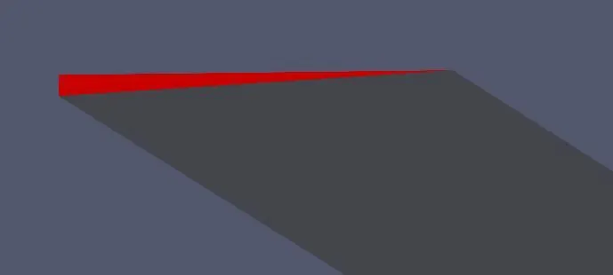
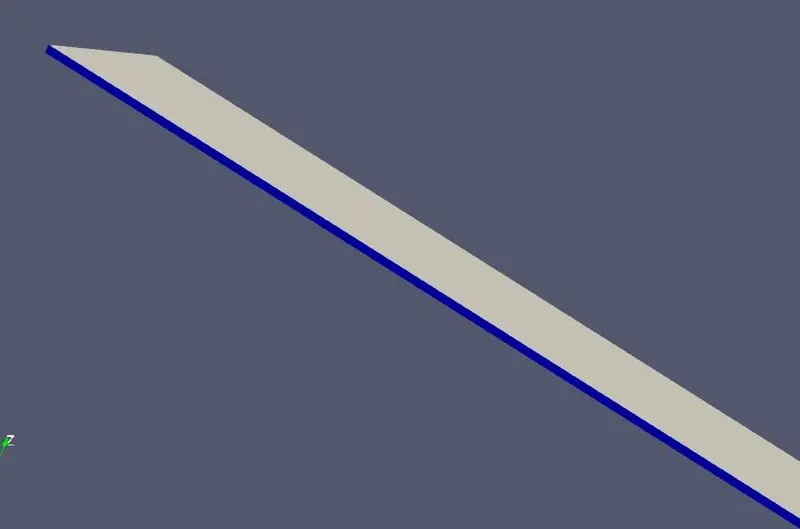
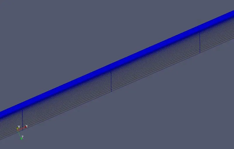
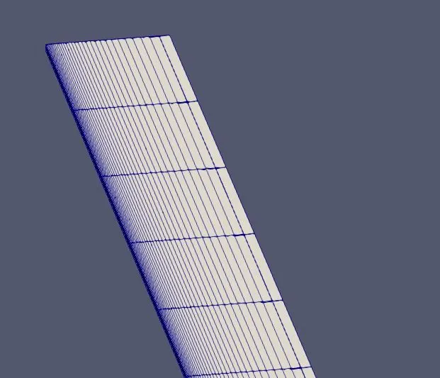
The objective of the challenge is to perform a simulation of flow through the pipe using the Open Foam tool Here we have taken a wedge shaped body to perform the simulation. A proper code has to be written in the block-Dict file to get the desired shape. The fluid used in the simulation is water at room temperature. The Flow is laminar in nature. For this condition, we use the icoFoam solver in OpenFoam to solve the case.
Entrance length:
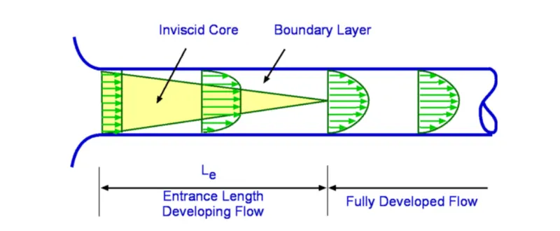
The length of the entrance is the distance that fluid travels after entering a pipe before the full development of the flow. Entrance length refers to the length of the entry region where effects from the pipe's interior wall spread as an expanding boundary layer into the flow. When the boundary layer extends to fill the entire pipe the flow grows into a fully developed flow where the flow characteristics no longer change with increased distance along the pipe. To define a variety of flow conditions, there are many different entrance lengths
Hydrodynamic entrance length:
The hydrodynamic entrance region refers to the area of a pipe where fluid entering a pipe develops a velocity profile due to viscous forces spreading from a pipe's interior wall. This region has a non-uniform flow. The fluid enters a pipe at a constant speed, sa fluid particles in the layer in contact with the pipe's surface come to a complete stop because of the no slip rule. The layer in contact with the pipe surface is resistant to the acceleration of neighboring layers due to viscous forces within the floid and slowly slows down adjacent layers of fluid, creating a velocity profile To keep the mass true the speed of the huid layers in the center of the pipe increases to compensate for the reduced speed of the fluid layers near the surface of the pipe. It creates a gradient of velocity across the pipe cross section
Entry length for the laminar flow is
Le = 0.05 x Re x D
Entry length for the laminar flow is
L= 4.4 x Re0.166 x D
To do the simulation we need to find properties using some variables. Those are Hagen Poiseuille equations.
Variables
Diameter D = 0.01
Radius, r= 0.005
Dynamic viscosity, mu= 0.00089 N/ m2
Density, mo = 997 kg/m2
Reyonids number, Re =2100
Hagen-Poiseuille equation
In non ideal fluid dynamic, the Hagen-Poiseuille equation, also known as the Hagen-Poiseuille Poiseuille law or Poiseuille equation, is a physical law that gives the pressure drop in an incompressible and Newtonian fluid in laminar flow flowing through a long cylindrical pipe of constant cross section.
Formulaes:
Average velcoity Vavrg=`(R_e * mu)/(rho*D)`
Maximum velocity Vmax=`2*V_avrg`
Pressure difference deltaP=`(8*mu*L*V_avrg)/(r^2)`
Kinematic pressure difference deltaPk=`(DeltaP)/rho`
Shear stress tau=`(2*mu*V_max*R)/r^2`
Program in OpenFoam:
BlockMeshdict:
/*--------------------------------*- C++ -*----------------------------------*\
  =========                 |
  \\      /  F ield         | OpenFOAM: The Open Source CFD Toolbox
   \\    /   O peration     | Website:  https://openfoam.org
    \\  /    A nd           | Version:  8
     \\/     M anipulation  |
\*---------------------------------------------------------------------------*/
FoamFile
{
    version     2.0;
    format      ascii;
    class       dictionary;
    object      blockMeshDict;
}
// * * * * * * * * * * * * * * * * * * * * * * * * * * * * * * * * * * * * * //

convertToMeters 1;

vertices
(
    (0 0 0)
    (0 4.9982866e-03 1.308847e-04)
    (0 4.9982866e-03 -1.308847e-04)
    (1.5 0 0)
    (1.5 4.9982866e-03 1.308847e-04)
    (1.5 4.9982866e-03 -1.308847e-04)
);

blocks
(
    hex (0 3 5 2 0 3 4 1) (500 50 1) simpleGrading (1 0.1 1)

 );

edges
(
   arc 1 2 (0 5.000000e-03 0)
   arc 4 5 (1.5 5.000000e-03 0)
);

boundary
(
    inlet
    {
        type patch;
        faces
        (
            (0 1 2 0)

        );
    }
    outlet
    {
        type patch;
        faces
        (
            (3 5 4 3)
        );
    }
    top
    {
        type wall;
        faces
        (
            (1 4 5 2)
        );
    }
     back
    {
        type wedge;
        faces
        (
            (0 2 5 3)
        );
    }
     front
    {
        type wedge;
        faces
        (
            (0 3 4 1)

        );
    }
    axis
    {
        type empty;
        faces
        (
            (0 3 3 0)

        );
    }
);

mergePatchPairs
(
);

// ************************************************************************* //
ControlDict:
/*--------------------------------*- C++ -*----------------------------------*\
  =========                 |
  \\      /  F ield         | OpenFOAM: The Open Source CFD Toolbox
   \\    /   O peration     | Website:  https://openfoam.org
    \\  /    A nd           | Version:  8
     \\/     M anipulation  |
\*---------------------------------------------------------------------------*/
FoamFile
{
    version     2.0;
    format      ascii;
    class       dictionary;
    location    "system";
    object      controlDict;
}
// * * * * * * * * * * * * * * * * * * * * * * * * * * * * * * * * * * * * * //

application     icoFoam;

startFrom       startTime;

startTime       0;

stopAt          endTime;

endTime         10;

deltaT          0.007;

writeControl    timeStep;

writeInterval   20;

purgeWrite      0;

writeFormat     ascii;

writePrecision  6;

writeCompression off;

timeFormat      general;

timePrecision   6;

runTimeModifiable true;


// ************************************************************************* //
Velocity:
/*--------------------------------*- C++ -*----------------------------------*\
  =========                 |
  \\      /  F ield         | OpenFOAM: The Open Source CFD Toolbox
   \\    /   O peration     | Website:  https://openfoam.org
    \\  /    A nd           | Version:  8
     \\/     M anipulation  |
\*---------------------------------------------------------------------------*/
FoamFile
{
    version     2.0;
    format      ascii;
    class       volVectorField;
    object      U;
}
// * * * * * * * * * * * * * * * * * * * * * * * * * * * * * * * * * * * * * //

dimensions      [0 1 -1 0 0 0 0];

internalField   uniform (0.187462 0 0);

boundaryField
{
    inlet
    {
        type            fixedValue;
        value           uniform (0.187462 0 0);
    }

    outlet
    {
        type            zeroGradient;
    }
    top
    {
        type           noSlip;
        value          uniform 0;
    }
    back
    {
        type            wedge;
    }
    front
    {
        type            wedge;
    }
    axis
    {
        type            empty;
    }
}

// ************************************************************************* //
Pressure:
/*--------------------------------*- C++ -*----------------------------------*\
  =========                 |
  \\      /  F ield         | OpenFOAM: The Open Source CFD Toolbox
   \\    /   O peration     | Website:  https://openfoam.org
    \\  /    A nd           | Version:  8
     \\/     M anipulation  |
\*---------------------------------------------------------------------------*/
FoamFile
{
    version     2.0;
    format      ascii;
    class       volScalarField;
    object      p;
}
// * * * * * * * * * * * * * * * * * * * * * * * * * * * * * * * * * * * * * //

dimensions      [0 2 -2 0 0 0 0];

internalField   uniform 0;

boundaryField
{
    inlet
    {
        type            zeroGradient;
    }

    outlet
    {
        type            fixedValue;
        value           uniform 0;
    }
    top
    {
        type            zeroGradient;

    }
    back
    {
        type            wedge;
    }
    front
    {
       type             wedge;
    }
    axis
    {
       type             empty;
    }
}

// ************************************************************************* //
Stepwise Procedure for creating the geometry file:
Firstly, we need to calculate the average velocity of the given fluid. For that we need to given inputs of Reynolds number, Diameter, Viscosity, and Density values.
1. Give proper header files that can generate the OpenFOAM header. Be very careful with parenthesis like commas, brackets and slash symbols which may lead us to errors.
2 Angles for the wedge has been given in the program.
3. Using all these values we calculate average Velocity. Maximum Velocity, Pressure Difference, and kinematic Pressure difference. The reason to calculate the kinematic pressure difference is in the OpenFOAM pressure file if we observe the units, units given are kinematic pressure.
4. The angle theta taken less than five degrees is because only one line has to pass through the center of the axis of symmetry
5. By using the file parsing technique, We need to write the Matlab code that can be useful to perform the simulations using different angles.
6. After getting the Block Mesh Dict file, copy it to the case setup file which is located in the run folder. Pressure, and Transport properties file which is obtained from the analytical solution means
7. Like this change other parameters like Velocity,pressure and transport properties file which is obtained from the analytical solution .
8. Now set the start and end time in the control-Dict file, and Mention the delta T values also.
9. Now place the command directory file in the cavity, run the file using command "block-Mesh".
10. The Above command gives us the mesh file.
11. Now check the mesh to see whether any error in mesh, Non-alignment and some other using 'checkMesh' command
12. Once the mesh check is over and success. Now use 'icoFoam' solver to run the case setup.
13. After running successfully, Use 'paraFoam' command to post-process the velocity and shear stress of the fluid.
Results:
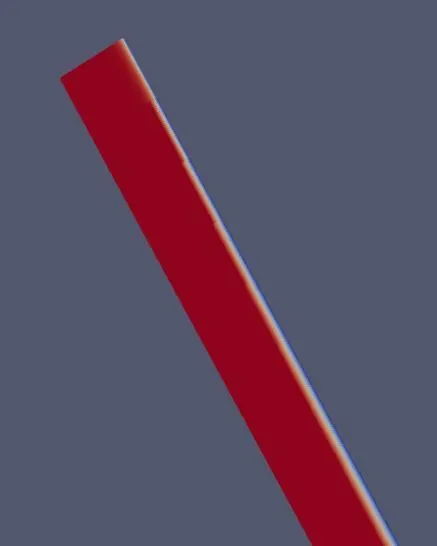
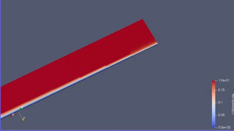
Generated geometry:
Velocity profiles at various distance:
Velocity profile at 0.01:
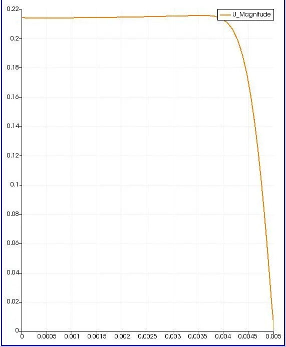
While observing the velcoity profile at entrance the flow is about to develop.
Velocity profile at 0.1:
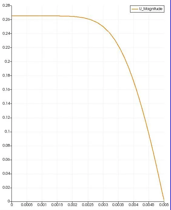
Velocity profile at 0.4:
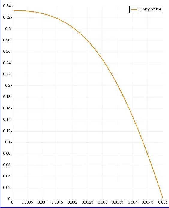
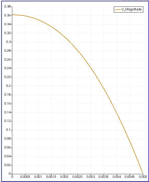
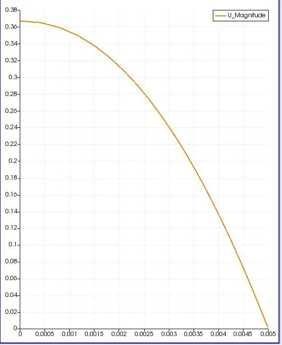
Likewise,if we observe the plots below the profile slowly becoming parabolic form.that means flow is developing slowly.
Velocity profile at 0.8:
Velocity profile at 1:
Velocity profile at 1.3:
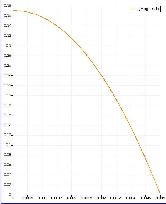
Velocity profile at 1.5:
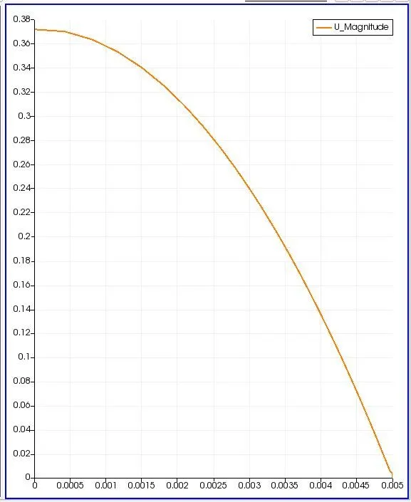
Now we can clearly see that the flow is fully developed.
Results:
Courant number mean =0.266202.
max=0.939381.
Execution time =143.21s.
clock time=192s.
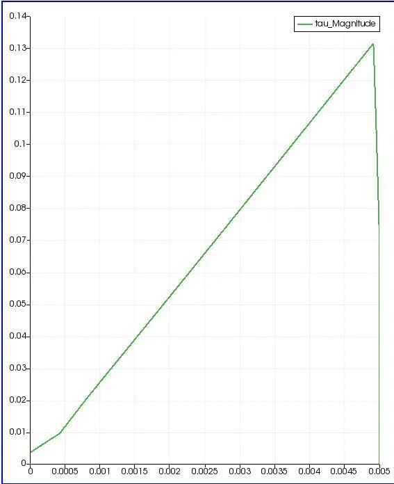
Shear stress Graph:
Comparing the results:
Maximum values velocity (m/sec) shear stress (N/m^2)
Analytical solution 0.374924 0.1334729
Numerical solution 0.37050 0.131000
Error % 1.17 1.85