Week 11 - Simulation of Flow through a pipe in OpenFoam
- Objective:
- Writing a program in MATLAB that can generate the computational mesh automatically for any wedge angle and grading schemes.
- Show that the velocity profile is fully developed.
- Post process velocity and shear stress Considering a cylindrical pipe with the working fluid water entering the pipe with the laminar flow. The aim is to simulate the flow through a section of pipe and compare the on with the Hagen Poiseuille's. equation.
2. Hagen Poiseuille’s Equation
- In nonideal fluid dynamics, the Hagen–Poiseuille equation, also known as the Hagen–Poiseuille law, is a physical law that gives the pressure drop in an incompressible and Newtonian fluid in laminar ow owing through a long cylindrical pipe of constant cross section. The pressure drop is given by:
`∆p=(32μLV)/D^2`
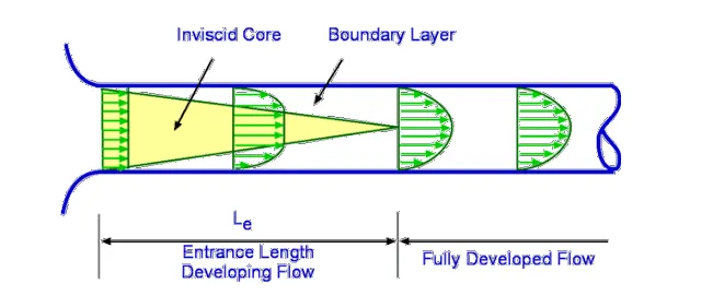
For a pipe with a laminar ow there are basically two regions. Entrance length developing region where the flow is not fully developed and the laminar flow layers are at equal velocity with respect to each other whereas in fully developed region the flow is fully developed and follows the Hagen–Poiseuille law.
Assumptions:
1) Geometry: Axi-symmetric
2) Reynolds number Re: 2100 (Laminar Flow)
3) Working Fluid; Water `( Density =997 (kg )/m^2 )`
4) Fluid temperature: `25 ℃`
5) Diameter of pipe = 0.02 m (R=0.01 m)
6) Dynamic viscosity =`0.890*10^(-3) pa.s`
7) Kinematic viscosity = `0.08927.10-6 m^2/s ∆p=(32μLV_(avg))/D^2`
8) theta = 4
and calculate the length of the pipe using entry length formula
L = 0.06*Re*d
= 0.06*2100*0.02
=2.52 meters.
Analytical Solution:
1. Average Velocity; `V_(avg)=(R_e μ)/(ρD)= 0.09373 m/s`
2. Maximum Velocity; `V_max=2.V_(avg)= 0.18746 m/s`
3. Pressure Drop = 16.817 pa
4. Kinematic Pressure Drop; `(∆p)/p= 0.016817 m`
Here for solving the problem numerically we will use the icoFoam solver with the cavity tutorial make the geometry along with the mesh and make the blockmeshDict le with the help of MATLAB as shown below
% Matlab Program for generating the blockMeshDict file for a wedge angle
clear all
close all
clc

% Given Inputs
% wedge angle
theta =4; % input('Enter the value of wedge angle = ');
Re = 2100;
D=0.02; %Diameter of the pipe
L = 0.06*Re*D; % Length of the pipe
R=D/2;
mu = 0.89e-3; %Viscosity of water at 25 deg C
rho = 997.0; % Densiy of water at 25 deg C
nu = mu/rho; % Kinematic viscosity of water at 25 deg C

% Calculation of pressure ans velocity
v_avg = Re*mu/(D*rho); %Average Velocity
v_max = 2*v_avg ; %Max Velocity
del_P = (32*mu*v_avg*L)/(D^2); % Pressure drop
kin_P = del_P/rho; % Kinematic Pressure drop

n1 = 50; % Number of cells along the pipe
n2 = 1; % Number of cells radially
n3 = 300; % Number of cells on the curve
gfactor=0.5;

% Vertices of the wedge
V0 = [0 0 0];
V1 = [0 R*cosd(theta/2) -R*sind(theta/2)];
V2 = [0 R*cosd(theta/2) R*sind(theta/2)];
V3 = [L 0 0];
V4 = [L R*cosd(theta/2) -R*sind(theta/2)];
V5 = [L R*cosd(theta/2) R*sind(theta/2)];

% Printing the file
text1='/*--------------------------------*- C++ -*----------------------------------*\';
text2=' ==========               |                                                    ';
text3=' \\       / F ield        | OPENFOAM: The Open Source CFD Toolbox              ';
text4='  \\     /  O peration    | Web: http://OpenFOAM.org                           ';
text5='   \\   /   A nd          | Version: 7                                         ';
text6='    \\ /    M anipulation |                                                    ';
text7='\*---------------------------------------------------------------------------*/';
text8='FoamFile                                                                       ';
text9='{                                                                              ';
text10='      version    2.0;                                                         ';
text11='      format     ascii;                                                       ';
text12='      class      dictionary;                                                  ';
text13='      object     blockMeshDict;                                               ';
text14='}                                                                             ';
text15='// * * * * * * * * * * * * * * * * * * * * * * * * * * * * * * * * * * * * * //';
text16='// * * * * * * * * * * * * * * * * * * * * * * * * * * * * * * * * * * * * * //';

% Creating file
f1 = fopen ('blockMeshDict.txt','wt')

fprintf(f1,'%s\n',text1);
fprintf(f1,'%s\n',text2);
fprintf(f1,'%s\n',text3);
fprintf(f1,'%s\n',text4);
fprintf(f1,'%s\n',text5);
fprintf(f1,'%s\n',text6);
fprintf(f1,'%s\n',text7);
fprintf(f1,'%s\n',text8);
fprintf(f1,'%s\n',text9);
fprintf(f1,'%s\n',text10);
fprintf(f1,'%s\n',text11);
fprintf(f1,'%s\n',text12);
fprintf(f1,'%s\n',text13);
fprintf(f1,'%s\n',text14);
fprintf(f1,'%s\n',text15);
fprintf(f1,'n');

fprintf(f1,'%s\n','convertToMeters 1;');

fprintf(f1,'%s\n','vertices');
fprintf(f1,'%s\n','(');
fprintf(f1,'%s (%f %f %f) \n',blanks(5),V0(1),V0(2),V0(3));
fprintf(f1,'%s (%f %f %f) \n',blanks(5),V1(1),V1(2),V1(3));
fprintf(f1,'%s (%f %f %f) \n',blanks(5),V2(1),V2(2),V2(3));
fprintf(f1,'%s (%f %f %f) \n',blanks(5),V3(1),V3(2),V3(3));
fprintf(f1,'%s (%f %f %f) \n',blanks(5),V4(1),V4(2),V4(3));
fprintf(f1,'%s (%f %f %f) \n',blanks(5),V5(1),V5(2),V5(3));
fprintf(f1,'%s\n',');');
fprintf(f1,'\n');

fprintf(f1,'%s\n','blocks');
fprintf(f1,'%s\n','(');
fprintf(f1,'%s %s\n',blanks(5),'hex (0 1 2 0 3 4 5 3) (50 1 200) simpleGrading (0.5 1 1)');
fprintf(f1,'%s\n',');');
fprintf(f1,'\n');

fprintf(f1,'%s\n','edges');
fprintf(f1,'%s\n','(');
fprintf(f1,'%s arc 1 2 (%f %f %f) \n',blanks(5),0,R,0);
fprintf(f1,'%s arc 4 5 (%f %f %f) \n',blanks(5),L,R,0);
fprintf(f1,'%s \n',');');
fprintf(f1,'\n');

fprintf(f1,'%s\n','boundary');
fprintf(f1,'%s\n','(');
fprintf(f1,'%s %s \n',blanks(5),'inlet');
fprintf(f1,'%s %s \n',blanks(5),'{');
fprintf(f1,'%s %s \n',blanks(10),'type patch;');
fprintf(f1,'%s %s \n',blanks(10),'faces');
fprintf(f1,'%s %s \n',blanks(10),'(');
fprintf(f1,'%s %s \n',blanks(15),'(0 1 2 0)');
fprintf(f1,'%s %s \n',blanks(10),');');
fprintf(f1,'%s %s \n',blanks(5),'}');

fprintf(f1,'%s %s \n',blanks(5),'outlet');
fprintf(f1,'%s %s \n',blanks(5),'{');
fprintf(f1,'%s %s \n',blanks(10),'type patch;');
fprintf(f1,'%s %s \n',blanks(10),'faces');
fprintf(f1,'%s %s \n',blanks(10),'(');
fprintf(f1,'%s %s \n',blanks(15),'(3 4 5 3)');
fprintf(f1,'%s %s \n',blanks(10),');');
fprintf(f1,'%s %s \n',blanks(5),'}');

fprintf(f1,'%s %s \n',blanks(5),'front');
fprintf(f1,'%s %s \n',blanks(5),'{');
fprintf(f1,'%s %s \n',blanks(10),'type wedge;');
fprintf(f1,'%s %s \n',blanks(10),'faces');
fprintf(f1,'%s %s \n',blanks(10),'(');
fprintf(f1,'%s %s \n',blanks(15),'(0 3 5 2)');
fprintf(f1,'%s %s \n',blanks(10),');');
fprintf(f1,'%s %s \n',blanks(5),'}');

fprintf(f1,'%s %s \n',blanks(5),'back');
fprintf(f1,'%s %s \n',blanks(5),'{');
fprintf(f1,'%s %s \n',blanks(10),'type wedge;');
fprintf(f1,'%s %s \n',blanks(10),'faces');
fprintf(f1,'%s %s \n',blanks(10),'(');
fprintf(f1,'%s %s \n',blanks(15),'(0 1 4 3)');
fprintf(f1,'%s %s \n',blanks(10),');');
fprintf(f1,'%s %s \n',blanks(5),'}');

fprintf(f1,'%s %s \n',blanks(5),'pipe');
fprintf(f1,'%s %s \n',blanks(5),'{');
fprintf(f1,'%s %s \n',blanks(10),'type wall;');
fprintf(f1,'%s %s \n',blanks(10),'faces');
fprintf(f1,'%s %s \n',blanks(10),'(');
fprintf(f1,'%s %s \n',blanks(15),'(1 4 5 2)');
fprintf(f1,'%s %s \n',blanks(10),');');
fprintf(f1,'%s %s \n',blanks(5),'}');

fprintf(f1,'%s %s \n',blanks(5),'axis');
fprintf(f1,'%s %s \n',blanks(5),'{');
fprintf(f1,'%s %s \n',blanks(10),'type empty;');
fprintf(f1,'%s %s \n',blanks(10),'faces');
fprintf(f1,'%s %s \n',blanks(10),'(');
fprintf(f1,'%s %s \n',blanks(15),'(0 3 3 0)');
fprintf(f1,'%s %s \n',blanks(10),');');
fprintf(f1,'%s %s \n',blanks(5),'}');
fprintf(f1,'%s \n',');');
fprintf(f1,'\n');

fprintf(f1,'%s \n','mergePatchPairs');

fprintf(f1,'%s \n','(');
fprintf(f1,'%s \n',');');

fprintf(f1,'\n');

fprintf(f1,'%s \n',text16);

fclose(f1);
The blockmeshDict file is thus created and is then replaced with the original blockmesh file in the system folder. The created blockmeshDict file can be seen below
/*--------------------------------*- C++ -*----------------------------------*\
  =========                 |
  \\      /  F ield         | OpenFOAM: The Open Source CFD Toolbox
   \\    /   O peration     | Website:  https://openfoam.org
    \\  /    A nd           | Version:  7
     \\/     M anipulation  |
\*---------------------------------------------------------------------------*/
FoamFile
{
    version     2.0;
    format      ascii;
    class       dictionary;
    object      blockMeshDict;
}
// * * * * * * * * * * * * * * * * * * * * * * * * * * * * * * * * * * * * * //

nconvertToMeters 1;

vertices
(
    (0.000000 0.000000 0.000000)
    (0.000000 0.009994 -0.000349)
    (0.000000 0.009994 0.000349)
    (2.520000 0.000000 0.000000)
    (2.520000 0.009994 -0.000349)
    (2.520000 0.009994 0.000349)
);

blocks
(
    hex (0 1 2 0 3 4 5 3) (50 1 200) simpleGrading (0.5 1 1)
);

edges
(
    arc 1 2 (0.000000 0.010000 0.000000)
    arc 4 5 (2.520000 0.010000 0.000000)
);

boundary
(
    inlet
    {
        type patch;
        faces
        (
            (0 1 2 0)
        );
    }
    outlet
    {
        type patch;
        faces
        (
            (3 4 5 3)
        );
    }
    front
    {
        type wedge;
        faces
        (
            (0 3 5 2)
        );
    }
    back
    {
        type wedge;
        faces
        (
            (0 1 4 3)
        );
    }
    pipe
    {
        type wall;
        faces
        (
            (1 4 5 2)
        );
    }
    axis
    {
        type empty;
        faces
        (
            (0 3 3 0)
        );
    }
);

mergePatchPairs
(
);

// ************************************************************************* //
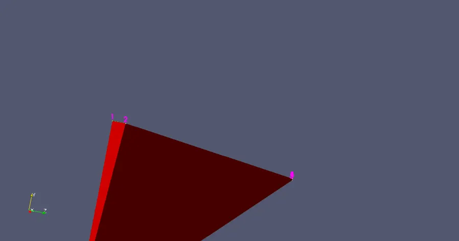
The created geometry can thus be seen in the figure below for the wedge angle of 4 degrees.
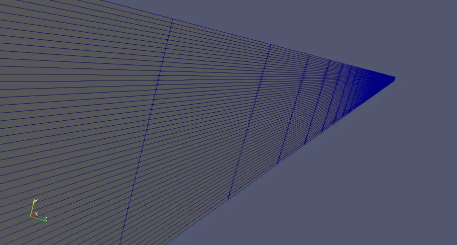
The axi-symmetric mesh generated can be seen below:
Further the initial and boundary conditions were further put in the problem as discussed above. The velocity Boundary condition can be seen below:
/*--------------------------------*- C++ -*----------------------------------*\
  =========                 |
  \\      /  F ield         | OpenFOAM: The Open Source CFD Toolbox
   \\    /   O peration     | Website:  https://openfoam.org
    \\  /    A nd           | Version:  7
     \\/     M anipulation  |
\*---------------------------------------------------------------------------*/
FoamFile
{
    version     2.0;
    format      ascii;
    class       volVectorField;
    object      U;
}
// * * * * * * * * * * * * * * * * * * * * * * * * * * * * * * * * * * * * * //

dimensions      [0 1 -1 0 0 0 0];

internalField   uniform (0 0 0);

boundaryField
{
   inlet
    {
        type            fixedValue;
        value           uniform (0.0937312 0 0);
    }

    outlet
    {
        type            zeroGradient;
        value           uniform 0.0168682;
    }

    pipe
    {
        type            noSlip;
    }

    axis
    {
        type            empty;
    }

    front
    {
        type            wedge;
    }

    back
    {
        type            wedge;
    }

}

// ************************************************************************* //
The pressure boundary conditions were put according to the pressure drop along the pipe as calculated above and can be seen below:
/*--------------------------------*- C++ -*----------------------------------*\
  =========                 |
  \\      /  F ield         | OpenFOAM: The Open Source CFD Toolbox
   \\    /   O peration     | Website:  https://openfoam.org
    \\  /    A nd           | Version:  7
     \\/     M anipulation  |
\*---------------------------------------------------------------------------*/
FoamFile
{
    version     2.0;
    format      ascii;
    class       volScalarField;
    object      p;
}
// * * * * * * * * * * * * * * * * * * * * * * * * * * * * * * * * * * * * * //

dimensions      [0 2 -2 0 0 0 0];

internalField   uniform 0;

boundaryField
{
    axis
    {
        type            empty;
    }

    pipe
    {
        type            zeroGradient;
    }

    inlet
    {
        type            zeroGradient;
    }

    outlet
    {
        type            fixedValue;
        value           uniform 0.0168682;
    }

    front
    {
        type            wedge;
    }

    back
    {
        type            wedge;
    }

}


// ************************************************************************* //
The kinematic viscosity values were put in the transproperties and can be seen below:
/*--------------------------------*- C++ -*----------------------------------*\
  =========                 |
  \\      /  F ield         | OpenFOAM: The Open Source CFD Toolbox
   \\    /   O peration     | Website:  https://openfoam.org
    \\  /    A nd           | Version:  7
     \\/     M anipulation  |
\*---------------------------------------------------------------------------*/
FoamFile
{
    version     2.0;
    format      ascii;
    class       dictionary;
    location    "constant";
    object      transportProperties;
}
// * * * * * * * * * * * * * * * * * * * * * * * * * * * * * * * * * * * * * //

nu              [0 2 -1 0 0 0 0] 0.000008927;


// ************************************************************************* //
Further the end time of the simulation was set to be 10 seconds and the time step i.e. Delta t was set to be 0.001 seconds as shown below:
/*--------------------------------*- C++ -*----------------------------------*\
  =========                 |
  \\      /  F ield         | OpenFOAM: The Open Source CFD Toolbox
   \\    /   O peration     | Website:  https://openfoam.org
    \\  /    A nd           | Version:  7
     \\/     M anipulation  |
\*---------------------------------------------------------------------------*/
FoamFile
{
    version     2.0;
    format      ascii;
    class       dictionary;
    location    "system";
    object      controlDict;
}
// * * * * * * * * * * * * * * * * * * * * * * * * * * * * * * * * * * * * * //

application     icoFoam;

startFrom       startTime;

startTime       0;

stopAt          endTime;

endTime         10;

deltaT          0.001;

writeControl    timeStep;

writeInterval   20;

purgeWrite      0;

writeFormat     ascii;

writePrecision  6;

writeCompression off;

timeFormat      general;

timePrecision   6;

runTimeModifiable true;


// ************************************************************************* //
After putting all these values, the simulation was run and the velocity contour at the last time step can be seen below:
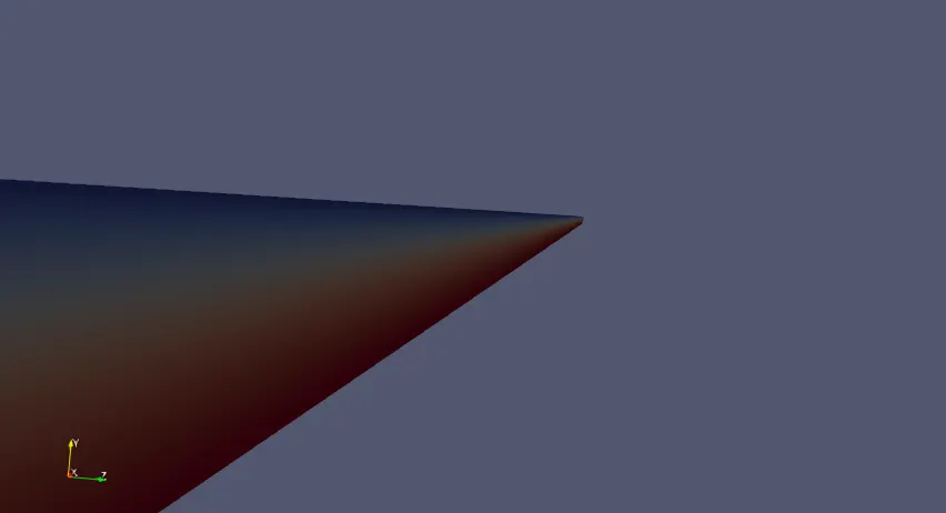
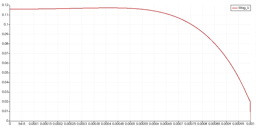
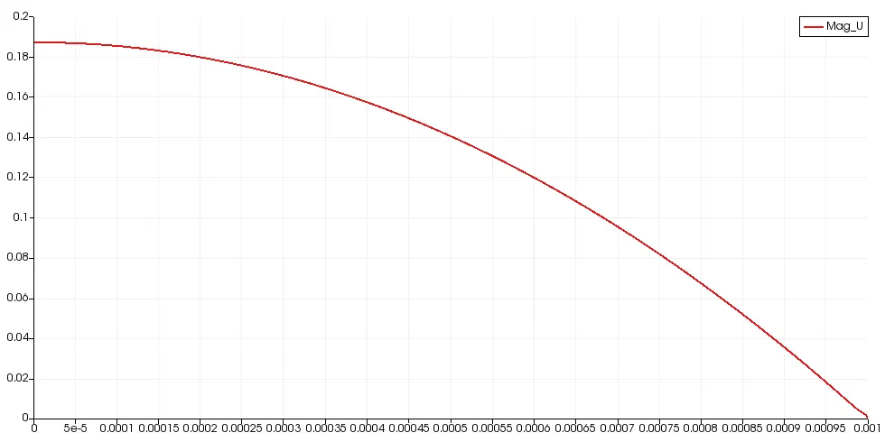
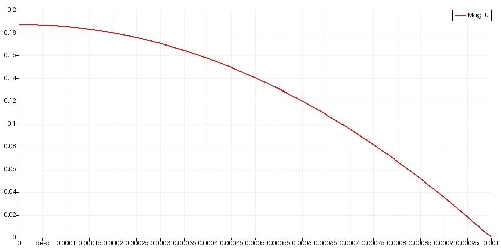
As this contour plot explains nothing the lines plots were used to get more precise and accurate results. The velocity plot was plotted at three different regions along the x and the velocity profile has been studied and can be seen below:
1. At a distance of 0.001m from inlet
2 .At a distance of 0.05m from inlet
3. At a distance of 0.15m from inlet
4. At outlet
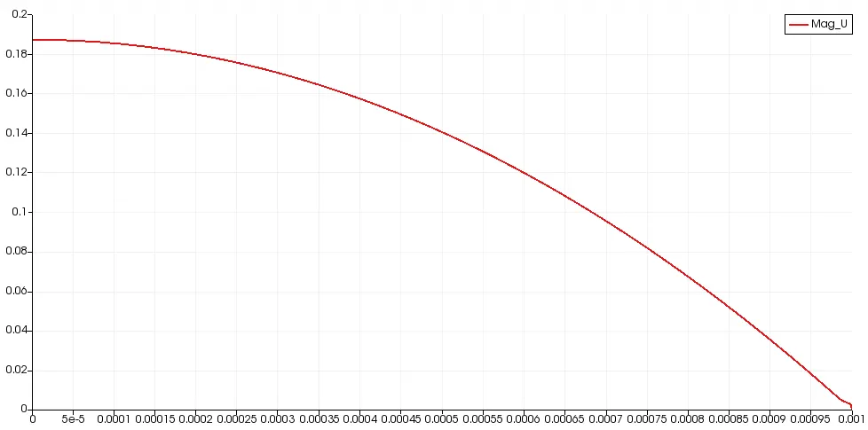
where y axis represents the velocity and x axis represents the length along the radius of the pipe. Here one thing can be noticed that near the walls of the pipe the velocity suddenly drops, this can be explained due to the no slip boundary conditions provided at the walls.
Further the shear stress was found out and the shear stress can be given as shown below:
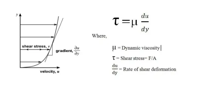
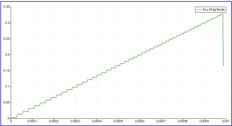
Here the formula suggests to multiply the dynamic viscosity with the gradient of velocity to and the shear stress thus it was done and the shear stress was plotted as shown below:
Conclusions:
- The HP equation was duly testified in this challenge as it can be seen in the velocity plots of the pipe at the end of the pipe near the outlet.
- At x=0.001 the velocity was seen slow and stable near the centre of the pipe this can be explained by the entrance length developing ow as explained above.
- Further it can be seen that the ow stats to develop with increase in length the prole becomes parabolic and fully developed ow can be seen in the end.
- At around x=0.15m the ow can be seen similar to that at the end of the ow, this shows that the fully developed region started almost at x=0.15m.
- The MATLAB program was successfully developed for BlockMesh le and was successfully executed and the data processing between the MATLAB and open foam was developed.
- In velocity plots it could be seen that the velocity dipped to the zero this is due to the no slip boundary condition.
- The shear stress plot also testifies the HP equation and law for the fully developed region.
- In shear stress plot irregularities can be observed along the plot this is due to the meshing because in FVM the values are measured along the surface and thus at the intersection of two nodes the value of the shear stress increases. Thus, this could be diminished by choosing the finer mesh, but it will also increase the computational time.