Week 11 - Simulation of Flow through a pipe in OpenFoam

INTRODUCTION

The pipe flow is a branch of fluid mechanics in which a fluid is passed through a closed conduit. The study of the flow through a pipe is very important in engineering since it has a very wide range of applications from power transmission to logistics. In many engineering devices, fluid power is transferred using pipes. Transport of oil and gas is through oil and gas pipelines, which connects different continents. So it is important to calculate the pressure losses and the power required for sustaining the flow through a pipe.

THEORY

For a laminar steady flow of a Newtonian fluid through a circular pipe, the pressure loss is can be calculated using the Hagen-Poiseuille equation. The flow through a pipe will become fully developed which means the velocity profile will not change after some initial length of the pipe, which is known as the hydrodynamic entry length which can be calculated using the formula:

\begin{equation}
\frac{L_{e}}{D} \approx 0.05 \text { Re }
\end{equation}

The analytical solution of the axisymmetric Navier-Stokes equation for a known value of pressure gradient gives the axial velocity distribution along the radial direction as shown below:

\begin{equation}
v_{x}=\left(-\frac{d p}{d x}\right) \frac{1}{4 \mu}\left(\frac{D^{2}}{4}-r^{2}\right)
\end{equation}

where `D` is the diameter of the pipe and `r` is the radial distance from the center of the pipe. This is the general solution of the flow through a circular pipe for `L >L_e` a parabolic velocity profile (Hagen-Poiseuille flow). Additionally, an interesting value to be computed is the maximum velocity corresponding to the vertex of the parabola, which is :

\begin{equation}
v_{x_{\max }}=\left(-\frac{d p}{d x}\right) \frac{D^{2}}{16 \mu}
\end{equation}

Where `\mu` is the dynamic viscosity of the fluid and `-\frac{d p}{d x}` is the pressure gradient along the direction of flow. For internal flow, the transition from laminar to turbulent happens at a Reynolds number of about Re ≈ 2300. Therefore, as the simulation is made for laminar flow, its physical properties will be set accordingly.

The pressure drop in a pipe when the flow is laminar can be calculated using the formula,

`\begin{equation} \Delta p = \frac{32\mu v_{avg}L}{D^2} \end{equation}`

The problem we are about to simulate is a flow through a pipe of diameter 0.02 m. The Reynolds number of the flow is assumed to be 100. The length of the pipe is set to be 0.3 m longer than the hydrodynamic entry length which depends on the Reynolds number. The dynamic viscosity of the fluid is assumed to be 0.89x`10^-3` Pas and density to be 997 `(kg)/m^3` which are properties of water at `25 ^\circC`. The velocity is selected such that the Reynolds number is 100. The equation of Reynolds number is as shown below:

`\begin{equation} Re = \frac{\rho V D}{\mu} \end{equation}`

The velocity van be then calculated to be `V = (\mu Re)/(\rho D) =(0.89 \times10^-3 \times100)/(997\times 0.02) = 0.0044634 m/s`

PREPROCESSING

The simulation of laminar pipe flow can be solved using icoFoam solver, The case directory will be named pipeFlow. A code is written in Matlab to generate the blockMeshdict for different values of wedge angle. The program in Matlab is shown below:

% Matlab script for generating the blockMeshDict file for a wedge angle
clear all
close all
clc

% Given Inputs
% wedge angle 

theta = 4;
Re = 100;

D=0.02; %Diameter of the pipe

Le = 0.06*Re*D% Length of the pipe

L = Le + 0.3

R=D/2;

mu = 0.89e-3; %Viscosity of water at 25 deg C

rho = 997.0; % Densiy of water at 25 deg C

nu = mu/rho; % Kinematic viscosity of water  at 25 deg C

% Calculation of pressure ans velocity 

v_avg = Re*mu/(D*rho) %Average Velocity
v_max = 2*v_avg  

%Max Velocity
del_P = (32*mu*v_avg*L)/(D^2) % Pressure drop
kin_P = del_P/rho % Kinematic Pressure drop
n1 = 50;  % Number of cells along the pipe
n2 = 1;   % Number of cells radially
n3 = 300; % Number of cells on the curve 

gfactor=0.5;
% Vertices of the wedge 
V0 = [0 0 0];
V1 = [0 R*cosd(theta/2) -R*sind(theta/2)];
V2 = [0 R*cosd(theta/2) R*sind(theta/2)];
V3 = [L 0 0];
V4 = [L R*cosd(theta/2) -R*sind(theta/2)];
V5 = [L R*cosd(theta/2) R*sind(theta/2)];

% Printing the file 
text1='/*-----------------------------*- C++ -*----------------------------*';
text2='  =========                |                                          ';
text3='  \      /  F ield        | OPENFOAM: The Open Source CFD Toolbox    ';
text4='   \    /   O peration    | Version: 7                               ';
text5='    \  /    A nd          | Web:   www.OpenFOAM.ORG                  ';
text6='     \/     M anipulation |                                          ';
text7='*------------------------------------------------------------------*/';
text8=' FoamFile';
text9='{';
text10='     version      2.0;';
text11='     format       ascii;';
text12='     class        dictionary;';
text13='     object       blockMeshDict;';
text14='}';
text15='// * * * * * * * * * * * * * * * * * * * * * * * * * * * * * * * * //';
text16='//*****************************************************************//';



% Creating file  
f1 = fopen('blockMeshDict.txt','wt');
fprintf(f1,'%s \n',text1);
fprintf(f1,'%s \n',text2);
fprintf(f1,'%s \n',text3);
fprintf(f1,'%s \n',text4);
fprintf(f1,'%s \n',text5);
fprintf(f1,'%s \n',text6);
fprintf(f1,'%s \n',text7);
fprintf(f1,'%s \n',text8);
fprintf(f1,'%s \n',text9);
fprintf(f1,'%s \n',text10);
fprintf(f1,'%s \n',text11);
fprintf(f1,'%s \n',text12);
fprintf(f1,'%s \n',text13);
fprintf(f1,'%s \n',text14);
fprintf(f1,'%s \n',text15);
fprintf(f1,'\n');fprintf(f1,'%s \n','convertToMeters 1;');
fprintf(f1,'%s \n','vertices');fprintf(f1,'%s \n','(');
fprintf(f1,'%s (%f %f %f) \n',blanks(5),V0(1),V0(2),V0(3));
fprintf(f1,'%s (%f %f %f) \n',blanks(5),V1(1),V1(2),V1(3));
fprintf(f1,'%s (%f %f %f) \n',blanks(5),V2(1),V2(2),V2(3));
fprintf(f1,'%s (%f %f %f) \n',blanks(5),V3(1),V3(2),V3(3));
fprintf(f1,'%s (%f %f %f) \n',blanks(5),V4(1),V4(2),V4(3));
fprintf(f1,'%s (%f %f %f) \n',blanks(5),V5(1),V5(2),V5(3));
fprintf(f1,'%s \n',');');
fprintf(f1,'\n');fprintf(f1,'%s \n','blocks');
fprintf(f1,'%s \n','(');
fprintf(f1,'%s %s \n',blanks(5),'hex (0 1 2 0 3 4 5 3) (50 1 200) simpleGrading (0.5 1 1)');
fprintf(f1,'%s \n',');');
fprintf(f1,'\n');
fprintf(f1,'%s \n','edges');
fprintf(f1,'%s \n','(');
fprintf(f1,'%s arc 1 2 (%f %f %f) \n',blanks(5),0,R,0);
fprintf(f1,'%s arc 4 5 (%f %f %f) \n',blanks(5),L,R,0);
fprintf(f1,'%s \n',');');fprintf(f1,'\n');
fprintf(f1,'%s \n','boundary');
fprintf(f1,'%s \n','(');
fprintf(f1,'%s %s \n',blanks(5),'inlet');
fprintf(f1,'%s %s \n',blanks(5),'{');
fprintf(f1,'%s %s \n',blanks(10),'type patch;');
fprintf(f1,'%s %s \n',blanks(10),'faces');
fprintf(f1,'%s %s \n',blanks(10),'(');
fprintf(f1,'%s %s \n',blanks(15),'(0 1 2 0)');
fprintf(f1,'%s %s \n',blanks(10),');');
fprintf(f1,'%s %s \n',blanks(5),'}');
fprintf(f1,'%s %s \n',blanks(5),'outlet');
fprintf(f1,'%s %s \n',blanks(5),'{');
fprintf(f1,'%s %s \n',blanks(10),'type patch;');
fprintf(f1,'%s %s \n',blanks(10),'faces');
fprintf(f1,'%s %s \n',blanks(10),'(');
fprintf(f1,'%s %s \n',blanks(15),'(3 4 5 3)');
fprintf(f1,'%s %s \n',blanks(10),');');
fprintf(f1,'%s %s \n',blanks(5),'}');
fprintf(f1,'%s %s \n',blanks(5),'front');
fprintf(f1,'%s %s \n',blanks(5),'{');
fprintf(f1,'%s %s \n',blanks(10),'type wedge;');
fprintf(f1,'%s %s \n',blanks(10),'faces');
fprintf(f1,'%s %s \n',blanks(10),'(');
fprintf(f1,'%s %s \n',blanks(15),'(0 3 5 2)');fprintf(f1,'%s %s \n',blanks(10),');');
fprintf(f1,'%s %s \n',blanks(5),'}');fprintf(f1,'%s %s \n',blanks(5),'back');
fprintf(f1,'%s %s \n',blanks(5),'{');fprintf(f1,'%s %s \n',blanks(10),'type wedge;');
fprintf(f1,'%s %s \n',blanks(10),'faces');fprintf(f1,'%s %s \n',blanks(10),'(');
fprintf(f1,'%s %s \n',blanks(15),'(0 1 4 3)');fprintf(f1,'%s %s \n',blanks(10),');');
fprintf(f1,'%s %s \n',blanks(5),'}');
fprintf(f1,'%s %s \n',blanks(5),'pipe');
fprintf(f1,'%s %s \n',blanks(5),'{');
fprintf(f1,'%s %s \n',blanks(10),'type wall;');
fprintf(f1,'%s %s \n',blanks(10),'faces');
fprintf(f1,'%s %s \n',blanks(10),'(');
fprintf(f1,'%s %s \n',blanks(15),'(1 4 5 2)');
fprintf(f1,'%s %s \n',blanks(10),');');
fprintf(f1,'%s %s \n',blanks(5),'}');
fprintf(f1,'%s %s \n',blanks(5),'axis');
fprintf(f1,'%s %s \n',blanks(5),'{');
fprintf(f1,'%s %s \n',blanks(10),'type empty;');
fprintf(f1,'%s %s \n',blanks(10),'faces');
fprintf(f1,'%s %s \n',blanks(10),'(');
fprintf(f1,'%s %s \n',blanks(15),'(0 3 3 0)');
fprintf(f1,'%s %s \n',blanks(10),');');
fprintf(f1,'%s %s \n',blanks(5),'}');
fprintf(f1,'%s \n',');');
fprintf(f1,'\n');
fprintf(f1,'%s \n','mergePatchPairs');
fprintf(f1,'%s \n','(');

fprintf(f1,'%s \n',');');
fprintf(f1,'\n');
fprintf(f1,'%s \n',text16);
fclose(f1);

The above code generates the blockMeshdict for a wedge angle of `4^\circ`. One this code is written the cylindrical wedge for any angle can be generated. The blockMeshdict file generated using the above code is shown below:

/*-----------------------------*- C++ -*----------------------------* 
  =========                |                                           
  \      /  F ield        | OPENFOAM: The Open Source CFD Toolbox     
   \    /   O peration    | Version: 7                                
    \  /    A nd          | Web:   www.OpenFOAM.ORG                   
     \/     M anipulation |                                           
*------------------------------------------------------------------*/ 
 FoamFile 
{ 
     version      2.0; 
     format       ascii; 
     class        dictionary; 
     object       blockMeshDict; 
} 
// * * * * * * * * * * * * * * * * * * * * * * * * * * * * * * * * // 

convertToMeters 1; 
vertices 
( 
      (0.000000 0.000000 0.000000) 
      (0.000000 0.009994 -0.000349) 
      (0.000000 0.009994 0.000349) 
      (0.420000 0.000000 0.000000) 
      (0.420000 0.009994 -0.000349) 
      (0.420000 0.009994 0.000349) 
); 

blocks 
( 
      hex (0 1 2 0 3 4 5 3) (50 1 200) simpleGrading (0.5 1 1) 
); 

edges 
( 
      arc 1 2 (0.000000 0.010000 0.000000) 
      arc 4 5 (0.420000 0.010000 0.000000) 
); 

boundary 
( 
      inlet 
      { 
           type patch; 
           faces 
           ( 
                (0 1 2 0) 
           ); 
      } 
      outlet 
      { 
           type patch; 
           faces 
           ( 
                (3 4 5 3) 
           ); 
      } 
      front 
      { 
           type wedge; 
           faces 
           ( 
                (0 3 5 2) 
           ); 
      } 
      back 
      { 
           type wedge; 
           faces 
           ( 
                (0 1 4 3) 
           ); 
      } 
      pipe 
      { 
           type wall; 
           faces 
           ( 
                (1 4 5 2) 
           ); 
      } 
      axis 
      { 
           type empty; 
           faces 
           ( 
                (0 3 3 0) 
           ); 
      } 
); 

mergePatchPairs 
( 
); 

//*****************************************************************// 

It is important to note that the inlet and outlet are given the wedge boundary condition.

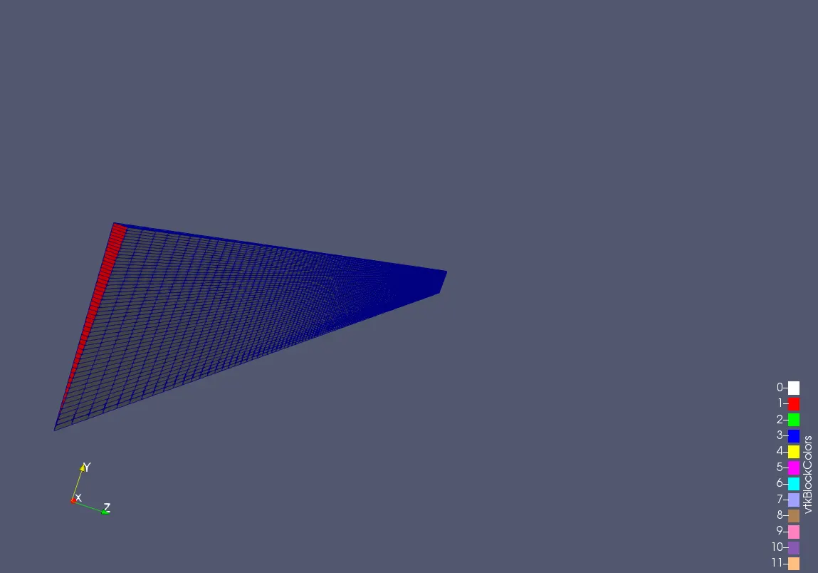
The mesh generated using the blockMesh utility can be visualised using paraview, which is shown below:

Boundary and initial condition

When solving the circulating internal flows it is important to set the inlet velocity and the outlet pressure. The inlet velocity was calculated to adjust the Reynolds number and the pressure drop can alsobe calculated using the Hagen-Poussiulie equation.

The velocity boundary and initial condition is shown below:

/*--------------------------------*- C++ -*----------------------------------*\
  =========                 |
  \\      /  F ield         | OpenFOAM: The Open Source CFD Toolbox
   \\    /   O peration     | Website:  https://openfoam.org
    \\  /    A nd           | Version:  8
     \\/     M anipulation  |
\*---------------------------------------------------------------------------*/
FoamFile
{
    version     2.0;
    format      ascii;
    class       volVectorField;
    object      U;
}
// * * * * * * * * * * * * * * * * * * * * * * * * * * * * * * * * * * * * * //

dimensions      [0 1 -1 0 0 0 0];

internalField   uniform (0.0044634 0 0);

boundaryField
{
    axis
    {
        type            empty;
    }

    inlet
    {
        type            fixedValue;
        value           uniform (0.0044634 0 0);
    }

    wall
    {
        type            noSlip;
       
    }

    outlet
    {
        type             zeroGradient;
        
    }

    front
    {
        type            wedge;
    }

    back
    {
        type          wedge;
     }
}
// ************************************************************************* //

The initial and boundary condition for pressure is set as shown below:

/*--------------------------------*- C++ -*----------------------------------*\
  =========                 |
  \\      /  F ield         | OpenFOAM: The Open Source CFD Toolbox
   \\    /   O peration     | Website:  https://openfoam.org
    \\  /    A nd           | Version:  8
     \\/     M anipulation  |
\*---------------------------------------------------------------------------*/
FoamFile
{
    version     2.0;
    format      ascii;
    class       volScalarField;
    object      p;
}
// * * * * * * * * * * * * * * * * * * * * * * * * * * * * * * * * * * * * * //

dimensions      [0 2 -2 0 0 0 0];

internalField   uniform 0;

boundaryField
{
    axis
    {
        type            empty;
    }

    inlet
    {
        type            zeroGradient;
    }

    wall
    {
        type            zeroGradient;
    }

    outlet
    {
        type            fixedValue;
        value           uniform 0;
    }

    front
    {
        type            wedge;
    }

    back
    {
        type           wedge;
     }
}

// ************************************************************************* //

Control

The control settings is as shown below:

/*--------------------------------*- C++ -*----------------------------------*\
  =========                 |
  \\      /  F ield         | OpenFOAM: The Open Source CFD Toolbox
   \\    /   O peration     | Website:  https://openfoam.org
    \\  /    A nd           | Version:  8
     \\/     M anipulation  |
\*---------------------------------------------------------------------------*/
FoamFile
{
    version     2.0;
    format      ascii;
    class       dictionary;
    location    "system";
    object      controlDict;
}
// * * * * * * * * * * * * * * * * * * * * * * * * * * * * * * * * * * * * * //

application     icoFoam;

startFrom       startTime;

startTime       0;

stopAt          endTime;

endTime         20;

deltaT          0.001;

writeControl    timeStep;

writeInterval   100;

purgeWrite      0;

writeFormat     ascii;

writePrecision  6;

writeCompression off;

timeFormat      general;

timePrecision   6;

runTimeModifiable true;


// ************************************************************************* //

POSTPROCESSING

RESULTS AND DISCUSSION

The velocity contours developed in the pipeflow simulation is shown below:

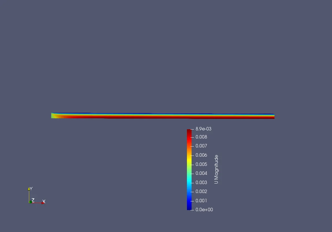
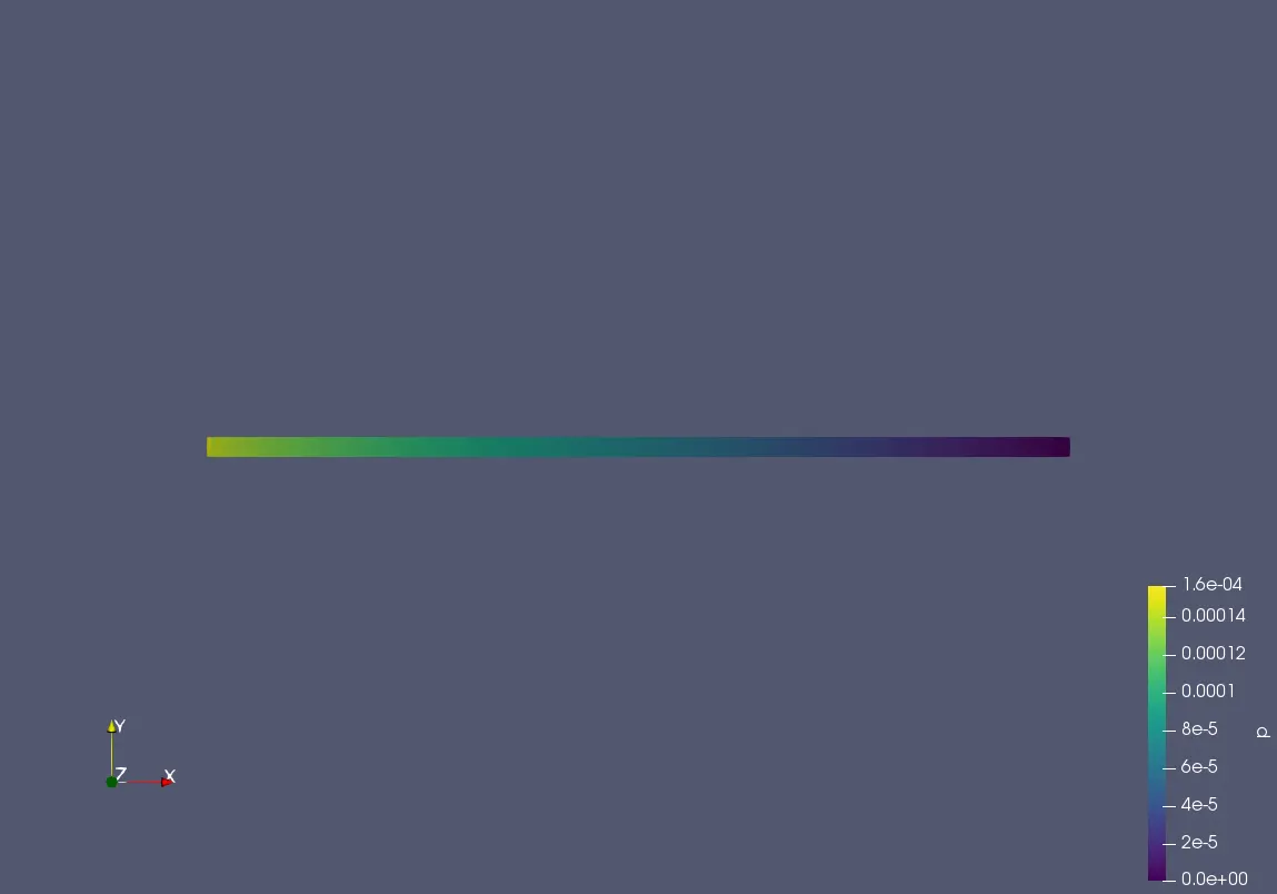
From the figure it can be seen that there is no change in the colour after a certain distance from the inlet which means that the flow has become fully developed. The velocity profile can be plotted to verify this. The pressure contour can also be visualised as shown below:

The velocity profile at different points along the axis of the pipe is plotted by extracting data from the simulation. The matplotlib library of python is used for postproccessing the data.The velocity profile along the different axial locations are given below:

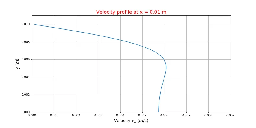
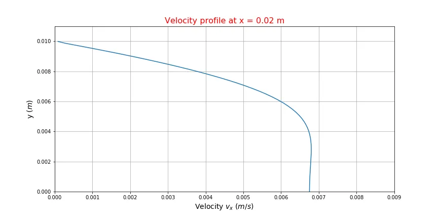
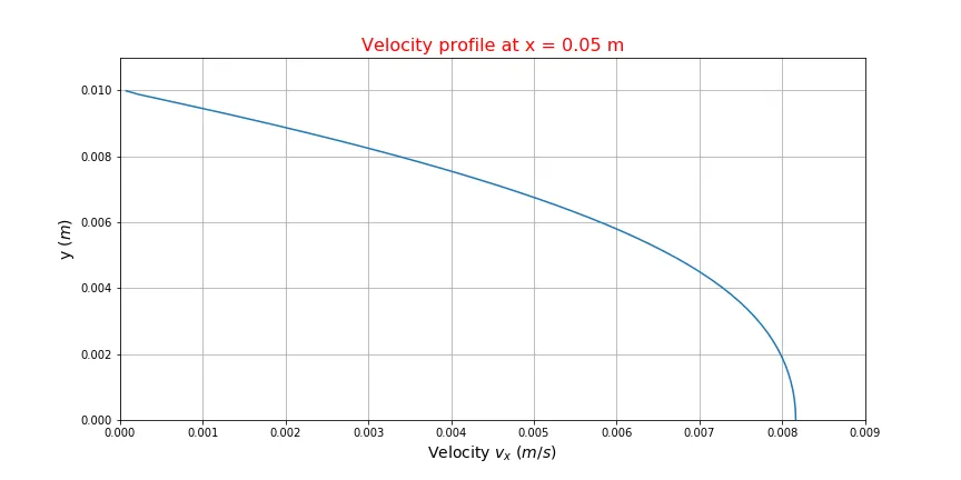
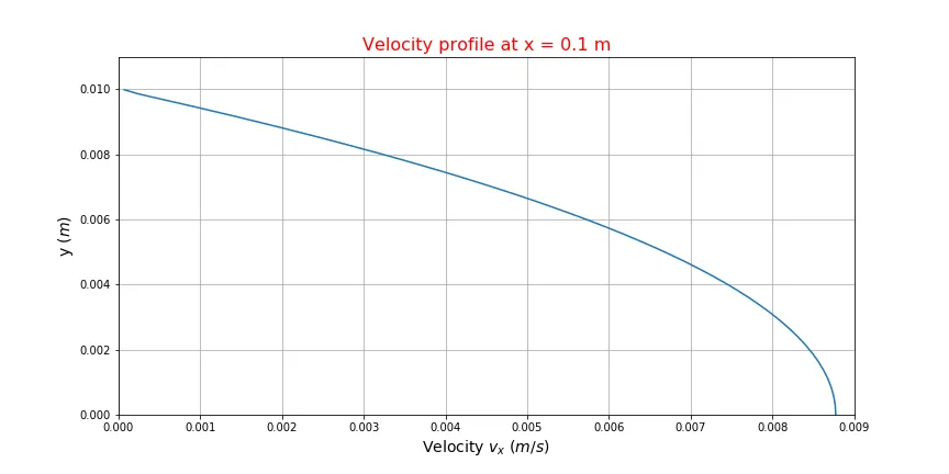
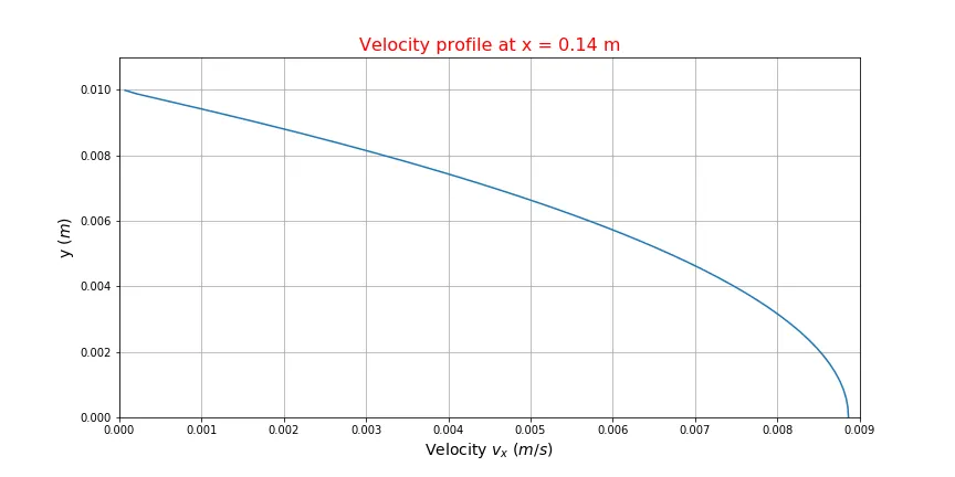
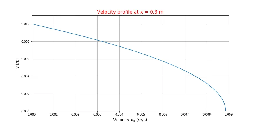
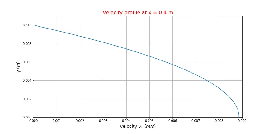
From analysing the above images it can be seen that at the entry region the velocity profileis developing. Once fully developed the velocity profile is not changing. It can be seen that the flow becomes fully developedat x = 0.1 m.

The pressure drop along the x axis is plotted in the next figure:

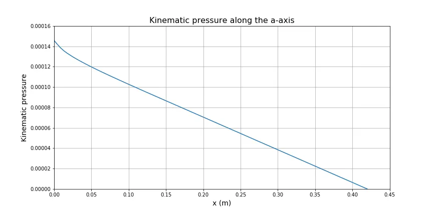
It can be seen that once the flow is fully developed, the pressure drop is linear. For a parabolic velocity profile the pressure drop must be linear, which is in agreement with the analytical solution. The shear stress distribution along the radial direction can be calculated using the paraview software. The mag() function can be used to calculate the magnitude of the vellocity vector U. The Gradient of unstructured data set filter can be used to calculate the gradient of magnitude of velocity mag(U). Then the calculator can be used to calculate the shear stress using the formula :

`\begin{equation} \tau = \mu \frac{du}{dy} \end{equation}`

The plot is generated using matplotlib library in python, the image is shown below:

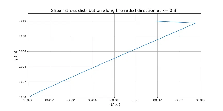
The shear stress distribution at the axial location at x = 0.3 m is linear and the maximum value of shear stress is at the walls of the pipe. The maximum value of the shear stress along the wall can be calculated for all the axial locations. The graph showing the shear stess distribution along the axis on the walls pf the pipe is shown below:

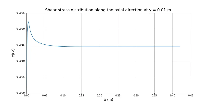
From this figure it is very easy to identify the entry length of the pipe. After the flow is fully developed the shear stress remains constant. The entry length from the above graph is 0.1 m. It is in agreement with the formula mentioned earlier.

From the analytical solution, the maximum velocity is twice the average velocity, i.e `v_{max} = 2\times v_{avg}`. The average velocity initialised in the simulation was 0.0044634 m/s. Therefore the maximum velocity for the analytival solution will be 0.0089268 m/s. From the simullation for the fully developed region the maximum velocity is 0.0088677m/s. So it is seen that there is an agreement between the simulated value and the analytical solution.

CONCLUSION

The laminar pipe flow at a Reynolds number = 100 is simulated using OpenFOAM. The blockMeshdict file is generated using a Matlab code.

Post-processing of the results is done using Paraview and Python.

The results are in good agreement with the analytical solution. The hydrodynamic entry length from the theoretical calculation and the numerical simulation was matched. It was visualised using the shear stress plot along the axis.

The velocity profile in the radial direction at different axial locations were plotted. After the flow is fully developed the velocity profile is parabolic. Once the flow is fully developed the velocity profile remains the same. Therefore the shear stress at the wall remains constant once the flow is fully developed.