Simulation of Flow through a pipe in OpenFoam
Objective:
Simulation of flow through the pipe. We need to calculate the length of the pipe using the entry length formula for laminar flow through a pipe,
Show that entry length is sufficient to produce a fully developed flow. Compare velocity profiles at different positions along the length of the pipe.
Show that the velocity profile matches with the Hagen Poiseuille's equation.
Theory:
Hagen Poiseuille's Law:
In nonideal fluid dynamics, the Hagen–Poiseuille equation, also known as the Hagen–Poiseuille law, is a physical law that gives the pressure drop in an incompressible and Newtonian fluid in laminar flow flowing through a long cylindrical pipe of constant cross-section. The assumptions of the equation are that the fluid is incompressible and Newtonian; the flow is laminar through a pipe of constant circular cross-section that is substantially longer than its diameter, and there is no acceleration of fluid in the pipe.
Flow inside a pipe:
Flow can be classified into 3 categories mainly:
- Laminar flow
- Transition
- Turbulent flow
The nature of fluid flow can be determined through its Reynold Number (Re) which for a flow through a pipe can be calculated by following formula:
`text( )Re= (rho*V_(avg)*D)/(mu)`
where,
`rho=text( density of fluid)`
`V_(avg)= text( Average velocity of fluid in pipe)`
`D=text( Diameter of pipe)`
`mu=text( Dynamic Viscosity of the fluid)`
The transition from laminar flow to turbulent flow occurs from laminar (`>=`Re 2100) to Transition(Re 2100- Re 4000) to turbulent (`<=`Re 4000) for smooth pipe with no viscous dissipation.
Hydrodynamic entry length:
The region from the pipe inlet to the point at which the velocity boundary layer merges at the centreline is called the hydrodynamic entrance region. The region beyond the entrance region in which the velocity profile is fully developed is called the fully developed region.
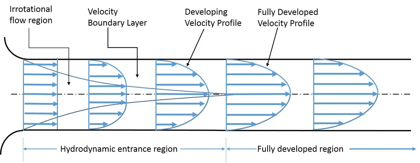
In laminar flow, the entry length is given approximately as:
`L_(text(laminar))~= 0.05*Re*D`
The hydrodynamic entrance region refers to the area of a pipe where fluid entering a pipe develops a velocity profile due to viscous forces spreading from a pipe's interior wall. This region has a non-uniform flow. The fluid enters a pipe at a constant speed, so fluid particles in the layer in contact with the pipe's surface come to a complete stop because of the no-slip rule. The layer in contact with the pipe surface is resistant to the acceleration of neighboring layers due to viscous forces within the fluid and slowly slows down adjacent layers of fluid, creating a velocity profile. To keep the mass true, the speed of the fluid layers in the center of the pipe increases to compensate for the reduced speed of the fluid layers near the surface of the pipe. It creates a gradient of velocity across the pipe cross-section.
The flow parameters are calculated using the following assumptions and formulas:
Reynold Number of flow: 2100
Diameter of pipe: 0.02 m
Angle of wedge: 4 degree
Working fluid: WATER
Density of working fluid at `25^o C= 997.05text( )Kg*m^(-3)`
Dynamic viscosity of fluid = 0.0008891 Pa.S
Kinematic Viscosity of fluid = `nu=mu/rho` `m^2s^-1`
Total length of pipe is assumed to be = `L_text(total)=L_text(laminar)+0.2` m = `2.1+0.2=2.3text( meters)`
Average velocity of fluid inside pipe = `V_(avg)=(Re*nu)/D` m/s
Maximum Velocity of fluid inside pipe = `V_(max)=2*V_(avg)` m/s
Pressure difference = `DeltaP= (32*mu*V_(avg)*L_text(total))/(D^2)` Pa
Kinematic Pressure = `DeltaP/rho` `m^2s^-2`
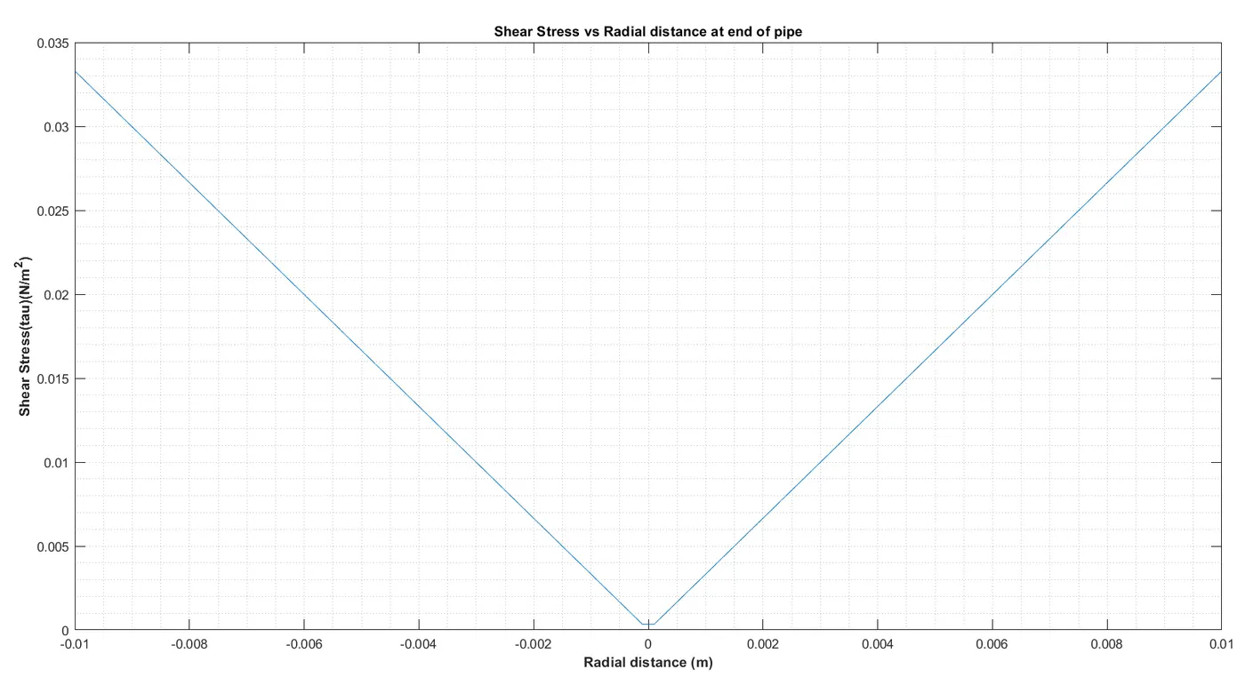
Shear stress = `tau=(2*mu*V_(max)*R)/(r^2)` `Nm^-2`
where, R = radial distance from axis & r = radius of pipe.
Main MATLAB program to generate blockMeshDict file:
clear all
close all
clc
% Input Parameters %
re= 2100; % Reynold's Number for perfectly laminar flow
d= 0.02; % Assuming diameter of pipe in meters
r=d/2; % Radius of pipe
theta= 4 % Wedge angle
mu=0.0008891; %Dynamic viscosity of water at 25 degree C, unit= Pa*S
rho=997.05; %Density of pure water at 25 degree C, kgm/m^3
nu= mu/rho; %Kinematic viscosity of water at 25 degree C, m^2/S

% Analytical calculation of Velocity,pressure and entrance length
L_e= 0.05*re*d; % Entrance length from inlet of pipe
L_t= L_e + 0.2 % Assumed Total length of pipe
v_avg= (re*nu)/d % Average velocity of water throughtout characteristic length
v_max= v_avg*2; % Max velocity of water at center of pipe characteristic length
Delta_P= (32*mu*v_avg*L_t)/(d^2) % Pressure Drop across pipe length
kp=Delta_P/rho %Kinematic pressure, m2/s2

%shear stress calculation in radial direction
R=linspace(-r,r,100);
for i=1:length(R)
   tau= (2*mu*v_max*abs(R))/(r^2);
end
figure(1)
plot(R,tau)
xlabel('Radial distance (m)')
ylabel('Shear Stress(tau)(N/m^2)')
title('Shear Stress vs Radial distance at end of pipe')
grid minor;

% Finding vertices
v0= [0 0 0];
v1= [0 r*cosd(theta/2) -r*sind(theta/2)];
v2= [0 r*cosd(theta/2) r*sind(theta/2)];
v3= [L_t 0 0];
v4= [L_t r*cosd(theta/2) -r*sind(theta/2)];
v5= [L_t r*cosd(theta/2) r*sind(theta/2)];

% Script to form blockMeshDict file.
f1= fopen('blockMeshDict.txt','w') % To create and write blockmesh file
fprintf(f1,'%s','/*--------------------------------*- C++ -*----------------------------------*');
fprintf(f1,'n========= |n');
fprintf(f1,' \\      / F ield        | OpenFOAM: The Open Source CFD Toolboxn');
fprintf(f1,'  \\    /  O peration    | Website:  https://openfoam.orgn');
fprintf(f1,'   \\  /   A nd          | Version:  8n');
fprintf(f1,'    \\/    M anipulation |n');
fprintf(f1,'%s','*---------------------------------------------------------------------------*/');
fprintf(f1,'nFoamFilen');
b1=blanks(5);
b2=blanks(6);
b3=blanks(7);
b4=blanks(4);
fprintf(f1,'{n');
fprintf(f1,'%s',' version',b1,'2.0;');
fprintf(f1,'n');
fprintf(f1,'%s',' format',b2,'ascii;');
fprintf(f1,'n');
fprintf(f1,'%s',' class',b3,'dictionary;');
fprintf(f1,'n');
fprintf(f1,'%s',' object',b2,'blockMeshDict;');
fprintf(f1,'n');
fprintf(f1,'}n');
fprintf(f1,'%s','// * * * * * * * * * * * * * * * * * * * * * * * * * * * * * * * * * * * * * //');
fprintf(f1,'nnconvertToMeters 1;nn');
% To form vertices
fprintf(f1,'verticesn');
fprintf(f1,'(n');
fprintf(f1,b4,'%s','(');
v_0= fprintf(f1,'(%f %f %f)   //vertice 0n',v0(1),v0(2),v0(3));
fprintf(f1,b4,'%s','(');
v_1= fprintf(f1,'(%f %f %f)   //vertice 1n',v1(1),v1(2),v1(3));
fprintf(f1,b4,'%s','(');
v_2= fprintf(f1,'(%f %f %f)   //vertice 2n',v2(1),v2(2),v2(3));
fprintf(f1,b4,'%s','(');
v_3= fprintf(f1,'(%f %f %f)   //vertice 3n',v3(1),v3(2),v3(3));
fprintf(f1,b4,'%s','(');
v_4= fprintf(f1,'(%f %f %f)   //vertice 4n',v4(1),v4(2),v4(3));
fprintf(f1,b4,'%s','(');
v_5= fprintf(f1,'(%f %f %f)   //vertice 5n',v5(1),v5(2),v5(3));
fprintf(f1,'n);n');
% To create blocks
fprintf(f1,'nblocksn');
fprintf(f1,'(n');
fprintf(f1,b4,'%s','(');
fprintf(f1,'%s','hex (0 1 2 0 3 4 5 3)');
% to create mesh
m1= input('Enter no. of mesh element along X-axis:')
m2= input('Enter no. of mesh element along Y-axis:')
m3= input('Enter no. of mesh element along Z-axis:')
fprintf(f1,blanks(1),'%s','(');
fprintf(f1,'(%3.0f %1.0f %3.0f)',m1,m2,m3);
fprintf(f1,'%s',' simpleGrading (1 1 1)');
fprintf(f1,'n);');
% To create edges
fprintf(f1,'nedgesn');
fprintf(f1,'(n');
fprintf(f1,'%s arc 1 2 (0 %f 0)',blanks(1),r);
fprintf(f1,'n%s arc 4 5 (%f %f 0)',blanks(1),L_t,r);
fprintf(f1,'n);nn');
% To apply boundary conditions
% For axis
fprintf(f1,'boundaryn(n');
fprintf(f1,'%s',' axis');
fprintf(f1,'n {n');
fprintf(f1,'%s',blanks(10),'type empty;');
fprintf(f1,'n');
fprintf(f1,'%s',blanks(10),'faces');
fprintf(f1,'n');
fprintf(f1,'%s',blanks(10),'(');
fprintf(f1,'n');
fprintf(f1,'%s',blanks(13),'(0 3 3 0)');
fprintf(f1,'n');
fprintf(f1,'%s',blanks(10),');');
fprintf(f1,'n }n');
% For fixedwalls
fprintf(f1,'%s',' fixedWalls');
fprintf(f1,'n {n');
fprintf(f1,'%s',blanks(10),'type wall;');
fprintf(f1,'n');
fprintf(f1,'%s',blanks(10),'faces');
fprintf(f1,'n');
fprintf(f1,'%s',blanks(10),'(');
fprintf(f1,'n');
fprintf(f1,'%s',blanks(13),'(2 1 4 5)');
fprintf(f1,'n');
fprintf(f1,'%s',blanks(10),');');
fprintf(f1,'n }n');
% For front
fprintf(f1,'%s',' front');
fprintf(f1,'n {n');
fprintf(f1,'%s',blanks(10),'type wedge;');
fprintf(f1,'n');
fprintf(f1,'%s',blanks(10),'faces');
fprintf(f1,'n');
fprintf(f1,'%s',blanks(10),'(');
fprintf(f1,'n');
fprintf(f1,'%s',blanks(13),'(1 0 3 4)');
fprintf(f1,'n');
fprintf(f1,'%s',blanks(10),');');
fprintf(f1,'n }n');
% For back
fprintf(f1,'%s',' back');
fprintf(f1,'n {n');
fprintf(f1,'%s',blanks(10),'type wedge;');
fprintf(f1,'n');
fprintf(f1,'%s',blanks(10),'faces');
fprintf(f1,'n');
fprintf(f1,'%s',blanks(10),'(');
fprintf(f1,'n');
fprintf(f1,'%s',blanks(13),'(2 5 3 0)');
fprintf(f1,'n');
fprintf(f1,'%s',blanks(10),');');
fprintf(f1,'n }n');
% For inlet
fprintf(f1,'%s',' inlet');
fprintf(f1,'n {n');
fprintf(f1,'%s',blanks(10),'type patch;');
fprintf(f1,'n');
fprintf(f1,'%s',blanks(10),'faces');
fprintf(f1,'n');
fprintf(f1,'%s',blanks(10),'(');
fprintf(f1,'n');
fprintf(f1,'%s',blanks(13),'(0 1 2 0)');
fprintf(f1,'n');
fprintf(f1,'%s',blanks(10),');');
fprintf(f1,'n }nn');
% For outlet
fprintf(f1,'%s',' outlet');
fprintf(f1,'n {n');
fprintf(f1,'%s',blanks(10),'type patch;');
fprintf(f1,'n');
fprintf(f1,'%s',blanks(10),'faces');
fprintf(f1,'n');
fprintf(f1,'%s',blanks(10),'(');
fprintf(f1,'n');
fprintf(f1,'%s',blanks(13),'(3 5 4 3)');
fprintf(f1,'n');
fprintf(f1,'%s',blanks(10),');');
fprintf(f1,'n }nn');
fprintf(f1,'n);n');
fprintf(f1,'nmergePatchPairs');
fprintf(f1,'n(n);nn');
fprintf(f1,'%s','// * * * * * * * * * * * * * * * * * * * * * * * * * * * * * * * * * * * * * //');
fclose(f1)

% To create and write flow data text file
f2= fopen('flow_data.txt','w')
fprintf(f2,'%s','/*--------------------------------*- C++ -*----------------------------------*');
fprintf(f2,'n========= |n');
fprintf(f2,' \\      / F ield        | OpenFOAM: The Open Source CFD Toolboxn');
fprintf(f2,'  \\    /  O peration    | Website:  https://openfoam.orgn');
fprintf(f2,'   \\  /   A nd          | Version:  8n');
fprintf(f2,'    \\/    M anipulation |n');
fprintf(f2,'n YOGBOT8 FLOW DATA PROPERTY CALCULATION FILEn');
fprintf(f2,'%s','*---------------------------------------------------------------------------*/');
fprintf(f2,'n n Reynold Number for the flow: %d',re);
fprintf(f2,'n Diameter of pipe: %.3f',d);
fprintf(f2,'n Angle of wedge: %d',theta);
fprintf(f2,'nn Fluid name: WATERn');
fprintf(f2,'n Density of fluid at 25C: %d',rho);
fprintf(f2,'n Dynamic Viscosity of fluid: %d',mu);
fprintf(f2,'n Kinematic Viscosity of fluid: %d',nu);
fprintf(f2,'n n Hydrodynamic entry length: %f',L_e);
fprintf(f2,'n Total length of pipe length: %f',L_t);
fprintf(f2,'nn no. of mesh element along X-axis: %d',m1);
fprintf(f2,'n no. of mesh element along Y-axis: %d',m2);
fprintf(f2,'n no. of mesh element along Z-axis: %d',m3);
fprintf(f2,'n n Average Velocity: %f',v_avg);
fprintf(f2,'n Maximum Velocity: %f',v_max);
fprintf(f2,'n n Pressure difference: %f',Delta_P);
fprintf(f2,'n Kinematic pressure: %f',kp);
dx=L_t/m3;
c=0.5; %courant number
dt=c*dx/v_avg;%time step size
et=L_t/v_avg;
fprintf(f2,'n n Time step size: %d',dt);
fprintf(f2,'n n End Time: %d',et);
fclose(f2)
blockMeshDict.txt file output:
/*--------------------------------*- C++ -*----------------------------------*
========= |
 \      / F ield        | OpenFOAM: The Open Source CFD Toolbox
  \    /  O peration    | Website:  https://openfoam.org
   \  /   A nd          | Version:  8
    \/    M anipulation |
*---------------------------------------------------------------------------*/
FoamFile
{
 version     2.0;
 format      ascii;
 class       dictionary;
 object      blockMeshDict;
}
// * * * * * * * * * * * * * * * * * * * * * * * * * * * * * * * * * * * * * //

convertToMeters 1;

vertices
(
    (0.000000 0.000000 0.000000)   //vertice 0
    (0.000000 0.009994 -0.000349)   //vertice 1
    (0.000000 0.009994 0.000349)   //vertice 2
    (2.300000 0.000000 0.000000)   //vertice 3
    (2.300000 0.009994 -0.000349)   //vertice 4
    (2.300000 0.009994 0.000349)   //vertice 5

);

blocks
(
    hex (0 1 2 0 3 4 5 3) ( 50 1 400) simpleGrading (1 1 1)
);
edges
(
  arc 1 2 (0 0.010000 0)
  arc 4 5 (2.300000 0.010000 0)
);

boundary
(
 axis
 {
          type empty;
          faces
          (
             (0 3 3 0)
          );
 }
 fixedWalls
 {
          type wall;
          faces
          (
             (2 1 4 5)
          );
 }
 front
 {
          type wedge;
          faces
          (
             (1 0 3 4)
          );
 }
 back
 {
          type wedge;
          faces
          (
             (2 5 3 0)
          );
 }
 inlet
 {
          type patch;
          faces
          (
             (0 1 2 0)
          );
 }

 outlet
 {
          type patch;
          faces
          (
             (3 5 4 3)
          );
 }


);

mergePatchPairs
(
);

// * * * * * * * * * * * * * * * * * * * * * * * * * * * * * * * * * * * * * //
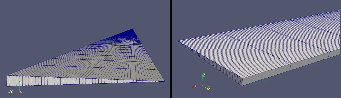
Generated mesh after using BlockMesh command:
flow_data.txt file output:
/*--------------------------------*- C++ -*----------------------------------*
 =========                |
 \      / F ield        | OpenFOAM: The Open Source CFD Toolbox
  \    /  O peration    | Website:  https://openfoam.org
   \  /   A nd          | Version:  8
    \/    M anipulation |

 YOGBOT8 FLOW DATA PROPERTY CALCULATION FILE
*---------------------------------------------------------------------------*/

 Reynold Number for the flow: 2100
 Diameter of pipe: 0.020
 Angle of wedge: 4

 Fluid name: WATER

 Density of fluid at 25C: 997.050000
 Dynamic Viscosity of fluid: 0.000889
 Kinematic Viscosity of fluid: 0.000001

 Hydrodynamic entry length: 2.100000
 Total length of pipe length: 2.300000

 no. of mesh element along X-axis: 50
 no. of mesh element along Y-axis:   1
 no. of mesh element along Z-axis: 400

 Average Velocity: 0.093632
 Maximum Velocity: 0.187263

 Pressure difference: 15.317624
 Kinematic pressure: 0.015363

 Time step size: 3.070541e-02
Pressure file:
/*--------------------------------*- C++ -*----------------------------------*
  =========                 |
  \  	  /  F ield         | OpenFOAM: The Open Source CFD Toolbox
   \	 /   O peration     | Website:  https://openfoam.org
    \  /    A nd           | Version:  8
     \/     M anipulation  |
*---------------------------------------------------------------------------*/
FoamFile
{
	version 	2.0;
	format  	ascii;
	class   	volScalarField;
	object  	p;
}
// * * * * * * * * * * * * * * * * * * * * * * * * * * * * * * * * * * * * * //

dimensions  	[0 2 -2 0 0 0 0];

internalField   uniform 0;

boundaryField
{
   axis
   {
  	 type        	empty;
   }
   fixedWalls
   {
  	 type        	zeroGradient;
   }
   front
   {
  	 type        	wedge;
   }
   back
   {
  	 type        	wedge;
   }
   inlet
   {
  	 type        	zeroGradient;
   }
   outlet
   {
  	 type        	fixedValue;
  	 value       	uniform 0.015363;
   }
}

// ************************************************************************* //
Velocity file:
/*--------------------------------*- C++ -*----------------------------------*
  =========                |
  \  	  / F ield     	   | OpenFOAM: The Open Source CFD Toolbox
   \	 /  O peration 	   | Website:  https://openfoam.org
    \  /   A nd       	   | Version:  8
     \/    M anipulation  |
*---------------------------------------------------------------------------*/
FoamFile
{
	version 	2.0;
	format  	ascii;
	class   	volVectorField;
	object  	U;
}
// * * * * * * * * * * * * * * * * * * * * * * * * * * * * * * * * * * * * * //

dimensions  	[0 1 -1 0 0 0 0];

internalField   uniform (0 0 0);

boundaryField
{
   axis
   {
  	 type        	empty;
   }
   fixedWalls
   {
  	 type        	noSlip;
   }
   front
   {
  	 type        	wedge;
   }
   back
   {
  	 type        	wedge;
   }
   inlet
   {
  	 type        	fixedValue;
  	 value       	uniform (0.093632 0 0);
   }
   outlet
   {
 		 type        	zeroGradient;
   }
}

// ************************************************************************* //
controlDict file:
/*--------------------------------*- C++ -*----------------------------------*
  =========                |
  \  	  / F ield     	   | OpenFOAM: The Open Source CFD Toolbox
   \	 /  O peration 	   | Website:  https://openfoam.org
    \  /   A nd       	   | Version:  8
     \/    M anipulation  |
*---------------------------------------------------------------------------*/
FoamFile
{
	version 	2.0;
	format  	ascii;
	class   	dictionary;
	location	"system";
	object  	controlDict;
}
// * * * * * * * * * * * * * * * * * * * * * * * * * * * * * * * * * * * * * //

application 	icoFoam;

startFrom   	startTime;

startTime   	0;

stopAt      	endTime;

endTime     	24.5;

deltaT      	3.070541e-03;

writeControl	timeStep;

writeInterval   20;

purgeWrite  	0;

writeFormat 	ascii;

writePrecision  6;

writeCompression off;

timeFormat  	general;

timePrecision   6;

runTimeModifiable true;


// ************************************************************************* //
TransportProperties file:
/*--------------------------------*- C++ -*----------------------------------*
  =========               |
  \      / F ield               | OpenFOAM: The Open Source CFD Toolbox
   \    /  O peration 	| Website:  https://openfoam.org
    \  /   A nd       	| Version:  8
     \/    M anipulation  |
*---------------------------------------------------------------------------*/
FoamFile
{
	version 	2.0;
	format  	ascii;
	class   	dictionary;
	location	"constant";
	object  	transportProperties;
}
// * * * * * * * * * * * * * * * * * * * * * * * * * * * * * * * * * * * * * //

nu          	[0 2 -1 0 0 0 0] 8.917e-7; //water at 25C

// ************************************************************************* //
Velocity contour at the initial and final stage of the simulation at the very start of the pipe:
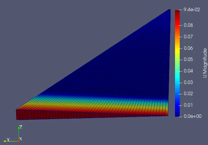
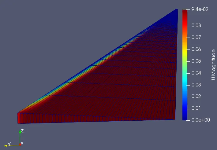
Fig: Initial condition at the start of the pipe Fig: Final condition at the start of the pipe
Final velocity Profile at different locations within the pipe:
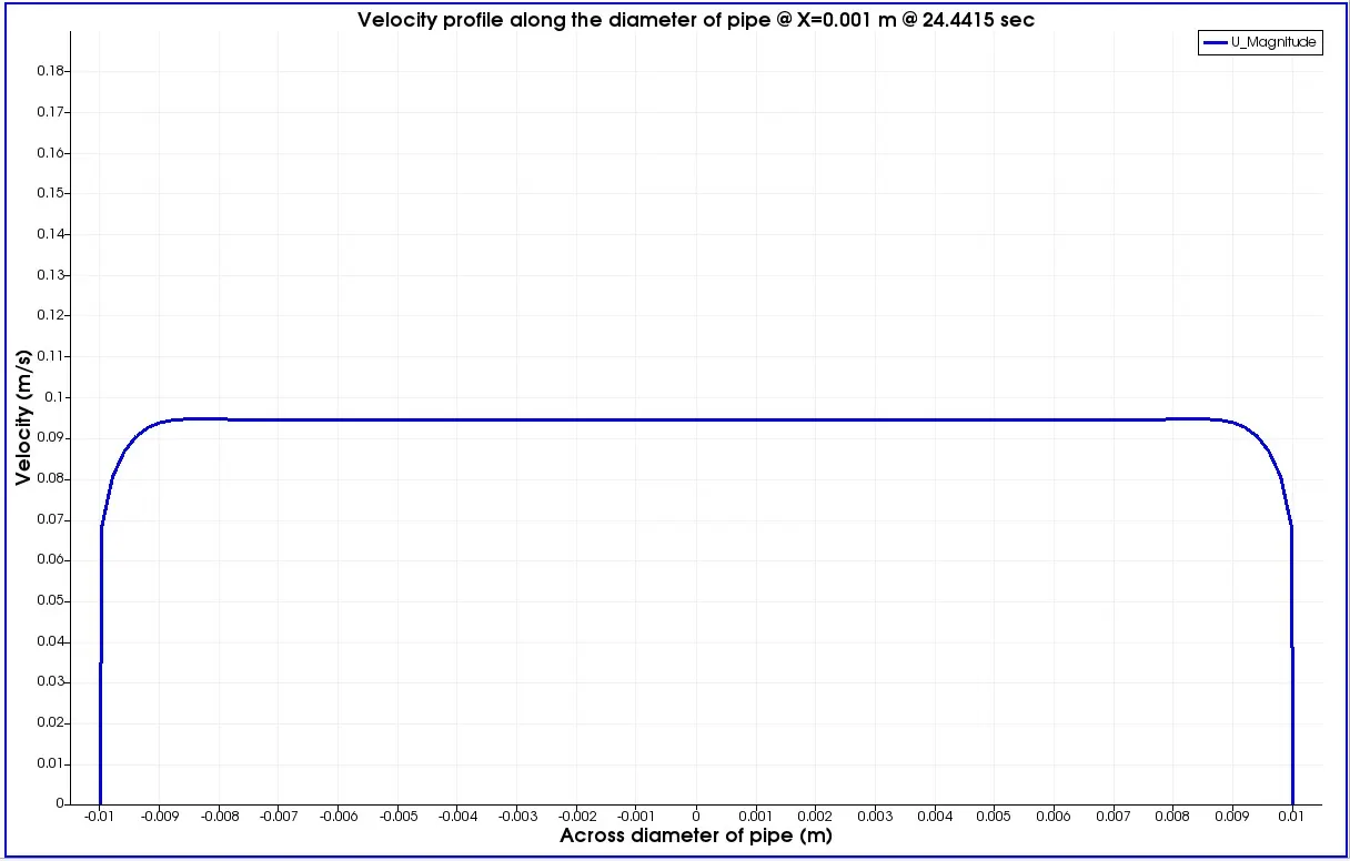
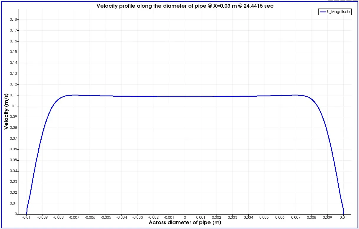
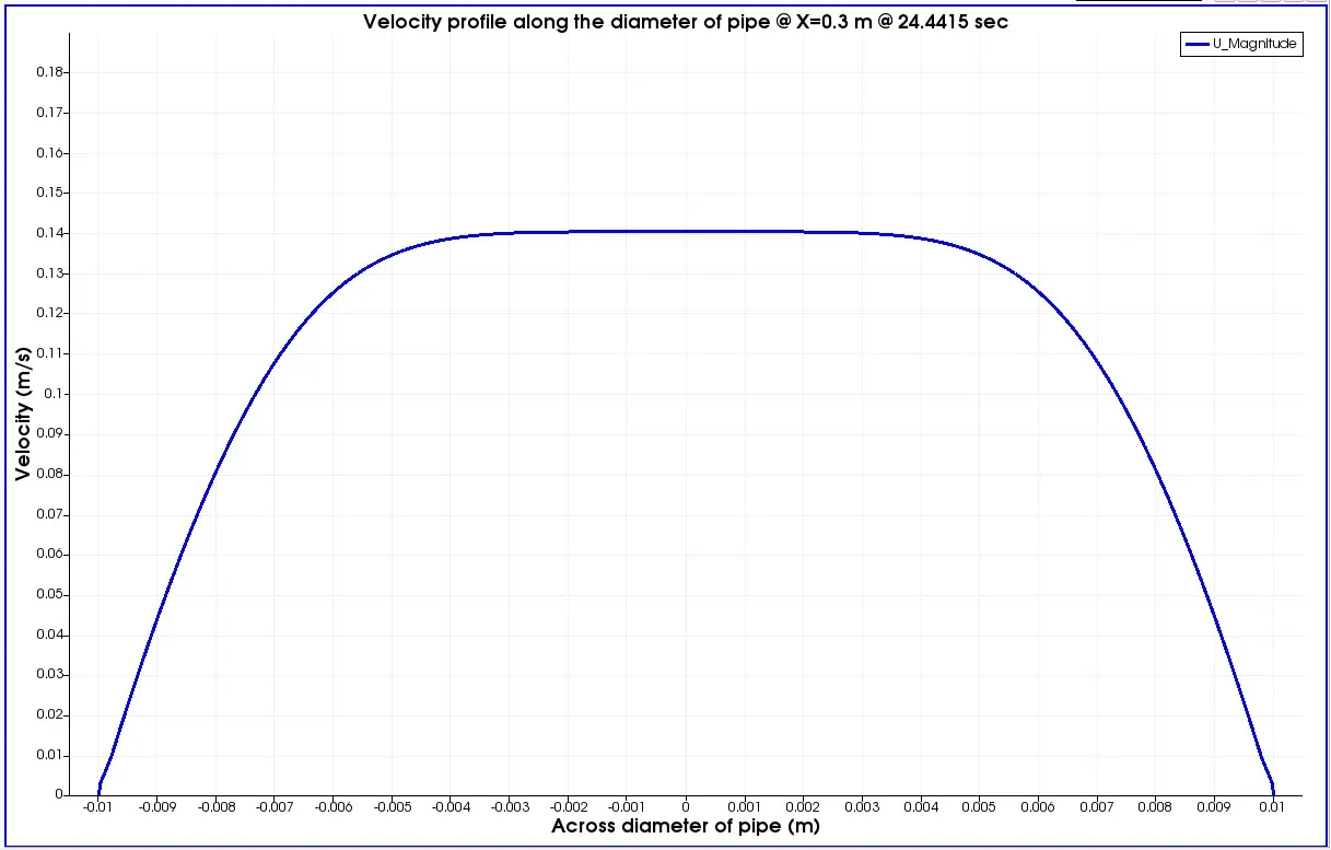
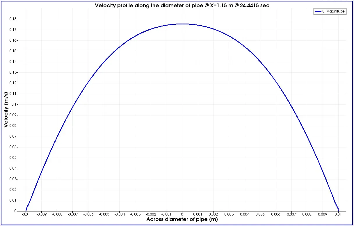
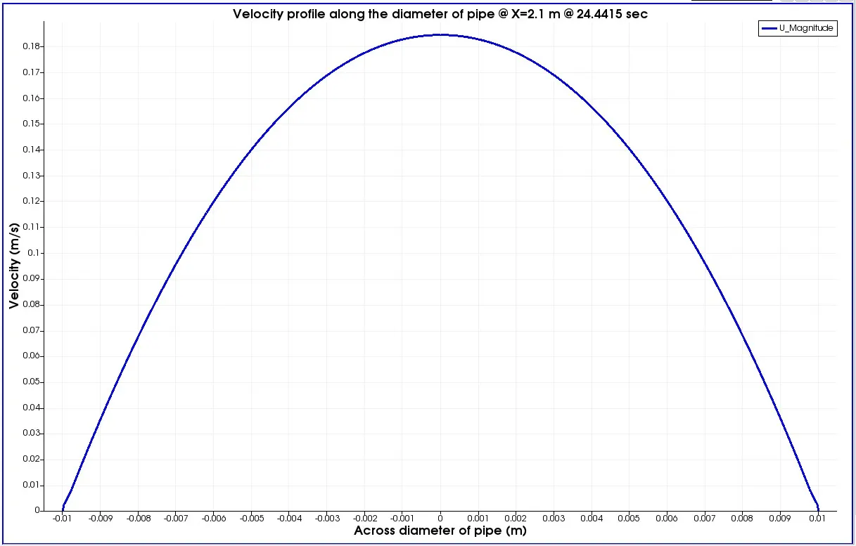
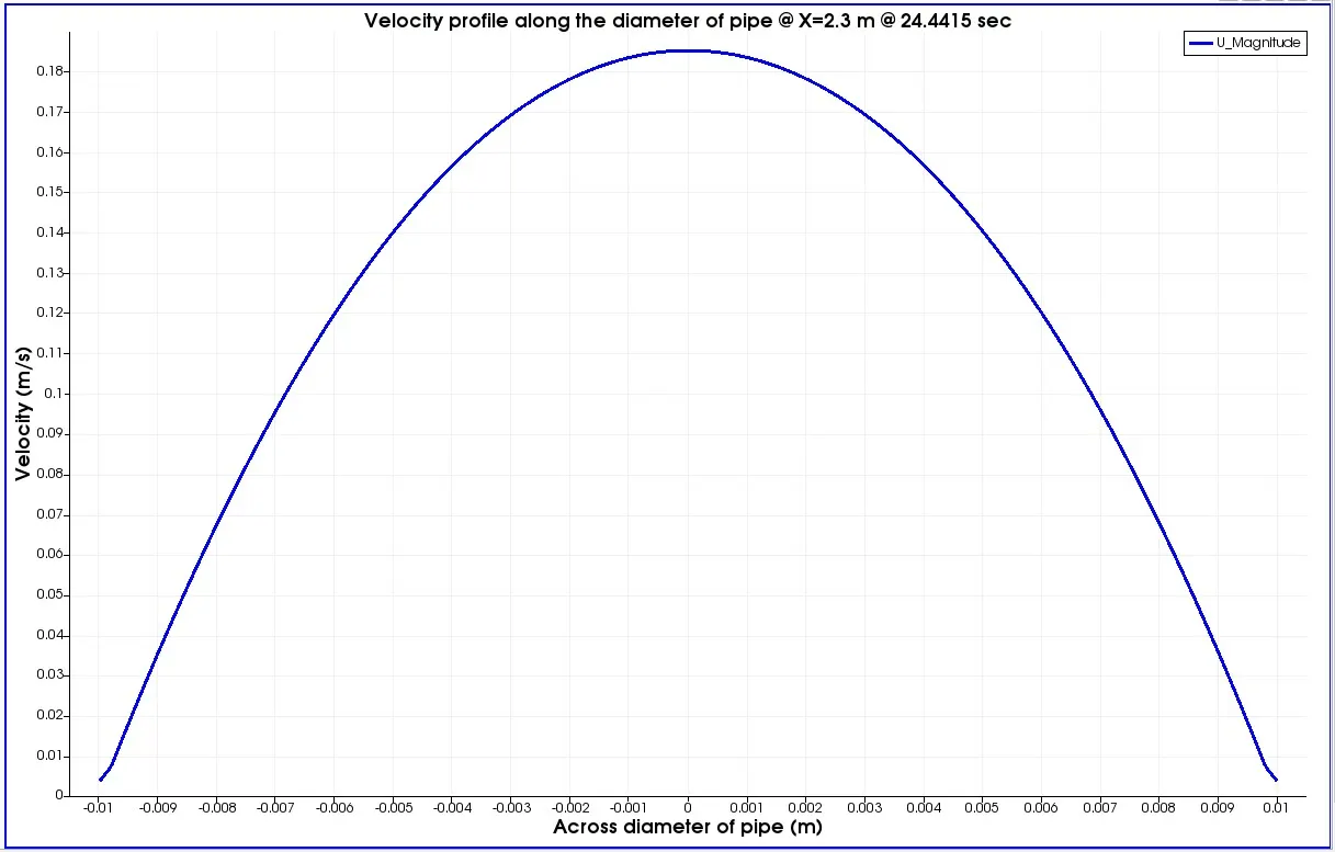
Change of velocity profile at the very end of the pipe from start to end of the simulation:
Shear Stress of the fully developed flow at the end of the pipe:
Conclusion:
It is evident from the results that after a certain distance the velocity profile starts taking shape of a parabolic path and becomes a perfect parabolic function after the has crossed hydrodynamic entry length, this profile remains unchanged in the axial direction which in turn tells us that the entry length we set up with respect to the conditions inside the domain is absolutely sufficient for obtaining the fully developed flow regime.
This proves the Hagen Poiseuille's flow can be achieved.