Week 11 - Simulation of Flow through a pipe in OpenFoam
Hagen- Poiseuille's equation
Given Rynolds no. of 2100 assumed for water as a fluid is nearly laminar flow. When fluid elements enter a pipe, due to friction force at the boundary of the pipe the crosssectional velocity is non uniform. Fluid elements flowing near the boundaries has less speed as compared to the center of the cross-section, giving rise to a velocity gradient across the cross-section of the pipe.
Hagen-Poiseuille's equation, derived from Hagen–Poiseuille law gives the pressure drop in an incompressible and Newtonian fluid in laminar flow flowing through a long cylindrical pipe of constant cross section.
Analytic Calulation
1. Average Velocity
`V = {Re * mu}/{D}`
2. Wall Shear Stress
`tau = {16*mu*V*R}/{D^2}`
3. Hydrodynamic Entrance Length
The hydrodynamic length is the length of the cross-sectional-area from the entrance where, a non changing velocity profile is created due to viscous forces from the interior of the wall of the pipe.
`Le = 0.06*Re*D`
4. Pressure Drop
`DeltaP = {32muVL}/{D^2}`
Where,
`mu` is the kinematic Viscosity
`D` is the pipe diameter
`Re` is the reynolds number
For analytical calculation of the velocity profile, below matlab script is developed with the declred properties.
clear all
close all
clc

% Theorical calculation with Hagen- Poiseuille's Equation

% Since the given liquid is water taking its properties and flow
% conditions are declared below:-
%% Geometry
% Diamter of pipe in m
D = 0.02;
% Angle
theta = 5;
%length of pipe
L = 3;

%% Declared Properties
% Given reynolds number
Re = 2100;
% Hydrodynamic-Entrance length
Le = 0.06*Re*D;
% Dynamic viscosity of water in NS/m^2
dynamicViscosity = 8.89e-4;
% Density in kg/m^3
rho = 997;

%% Calculated Properties
% Calculating Kinematic Viscosity in m^2/S
mU = dynamicViscosity/rho;
% Calculating Average Velocity in m/s
vAvg = (Re*mU)/D;
% Calculating MaximUm velocity in m/s
vMax = 2*vAvg;
% Calculating Kinematic Pressure Drop in N/m^2
dP = (32*mU*vAvg*L)/(D^2);
% Radius Array
R = linspace(0,0.01,20);

for i = 1:length(R)
    % Radial velocity Distribution
    vLocal(i) = 2*vAvg*(1-(4*R(i)^2/D^2));

    % Wall shear stress
    tau(i) = (16*mU*rho*vAvg*R(i))/D^2;
end
%% Plotting
figure(1)
subplot(1,2,1)
plot(R,vLocal, 'linewidth', 2, 'color', 'r')
xlabel('Radial Distance')
ylabel('Pipe Velocity Distribution')
legend('Theoretical Velocity')
% Shear Stress plot
subplot(1,2,2)
plot(R,tau, 'linewidth', 2, 'color', 'r')
xlabel('Radial Distance')
ylabel('Wall Shear Stress')
legend('Theoretical Wall Shear Stress')
sgtitle("Analytical Calculations")
The velocity plot and shear stress plot using the Hp equations are as below:-
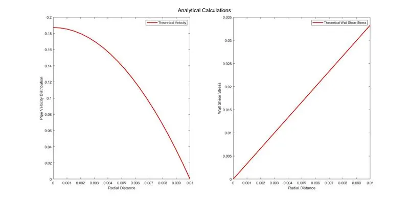
The maximum velocity in the center of the pipe is 0.1873.
Simulation
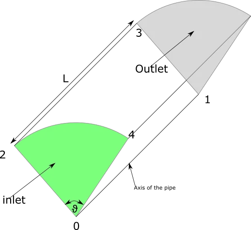
Boundary names and geometry for simulating the pipe flow is described below:-
The inlet boundary condition for velocity is calculated using the equaiton:-
for velocity in the inlet = `(Re*mu)/D`
where, `mu` is the Kinematic Viscosity
D is the Diameter of the pipe.
The Pressure Boundary condition on the outlet region is calculated using :-
`(32*mu*V*L)/(D^2)`
V = average velocity
D = Diameter of the pipe
L = Length of the pipe
mu = kinematic viscosity
The simulation is carried using the Diameter as 0.02 m, L = 3m, theta as 5 deg.
The matlab script for creating the blockMeshDict file is :-
% Matlab script for generating the blockMeshDict file given wedge angle
clear all
close all
clc

%% Properties declaration
% User input wedge Angle
theta = input(' Enter the value of wedge angle in degrees: ');

% Assumed Diameter of the pipe
D = input(' Enter the value of pipe diameter in m: ');

%L = 0.06*Re*D; % Length of the pipe

% User input Length
L = input('\n Enter the value of Length of Pipe in m: ');
% Radius of the Pipe
R=D/2;

% No. of cells along the radial direction
N1 = 100;
% No. of cells along the circumferential direction
N2 = 1;
% No. of cells along the length direction
N3 = 300;

%% Wedge fomation
% Center of the pipe
v0 = [0 0 0];
% Vertices on the circumference of the pipe
vc01 = [0 R*cosd(theta/2) -R*sind(theta/2)];
vc02 = [0 R*cosd(theta/2) R*sind(theta/2)];

% Corresponding Vertices on the other side of the pipe
v1 = [L 0 0];
vc11 = [L R*cosd(theta/2) -R*sind(theta/2)];
vc12 = [L R*cosd(theta/2) R*sind(theta/2)];


% Header of the file
file_type=' FoamFile';
% Header Dictionary
Dl1='{';
Dl2='    version     2.0;';
Dl3='    format      ascii;';
Dl4='    class       dictionary;';
Dl5='    object      blockMeshDict;';
Dl6='}';
% Creating file
file = fopen('blockMeshDict','wt');

fprintf(file,'%s\n',file_type);
fprintf(file,'%s\n',Dl1);
fprintf(file,'%s\n',Dl2);
fprintf(file,'%s\n',Dl3);
fprintf(file,'%s\n',Dl4);
fprintf(file,'%s\n',Dl5);
fprintf(file,'%s\n',Dl6);
fprintf(file,'\n');

fprintf(file,'%s\n','convertToMeters 1;');
%% Geometry Declaration
% Declaring the Vertices
fprintf(file,'%s\n','vertices');
fprintf(file,'%s\n','(');

fprintf(file,'%s (%f %f %f) \n',blanks(5),v0(1),v0(2),v0(3)); % vertex 0
fprintf(file,'%s (%f %f %f) \n',blanks(5),v1(1),v1(2),v1(3)); % vertex 1
fprintf(file,'%s (%f %f %f) \n',blanks(5),vc01(1),vc01(2),vc01(3)); % vertex 2
fprintf(file,'%s (%f %f %f) \n',blanks(5),vc11(1),vc11(2),vc11(3)); % vertex 3
fprintf(file,'%s (%f %f %f) \n',blanks(5),vc02(1),vc02(2),vc02(3)); % vertex 4
fprintf(file,'%s (%f %f %f) \n',blanks(5),vc12(1),vc12(2),vc12(3)); % vertex 5
fprintf(file,'%s\n',');');
fprintf(file,'\n');

% Declaring the Wedge block
fprintf(file,'%s\n','blocks');
fprintf(file,'%s\n','(');
fprintf(file,'%s %s %d %d %d %s\n',blanks(5),'hex (0 2 4 0 1 3 5 1) (',N1,N2,N3,') simpleGrading (0.5 1 1)');
fprintf(file,'%s\n',');');
fprintf(file,'\n');

% Declaring the arc edges
fprintf(file,'%s\n','edges');
fprintf(file,'%s\n','(');
fprintf(file,'%s arc 2 4 (%f %f %f) \n',blanks(5),0,R,0);
fprintf(file,'%s arc 3 5 (%f %f %f) \n',blanks(5),L,R,0);
fprintf(file,'%s \n',');');
fprintf(file,'\n');

% Declaring the boundary names
fprintf(file,'%s\n','boundary');
fprintf(file,'%s\n','(');
% Input Flow face
fprintf(file,'%s %s \n',blanks(5),'inlet_flow');
fprintf(file,'%s %s \n',blanks(5),'{');
fprintf(file,'%s %s \n',blanks(10),'type patch;');
fprintf(file,'%s %s \n',blanks(10),'faces');
fprintf(file,'%s %s \n',blanks(10),'(');
fprintf(file,'%s %s \n',blanks(15),'(0 2 4 0)');
fprintf(file,'%s %s \n',blanks(10),');');
fprintf(file,'%s %s \n',blanks(5),'}');

% Outlet flow face
fprintf(file,'%s %s \n',blanks(5),'outlet_flow');
fprintf(file,'%s %s \n',blanks(5),'{');
fprintf(file,'%s %s \n',blanks(10),'type patch;');
fprintf(file,'%s %s \n',blanks(10),'faces');
fprintf(file,'%s %s \n',blanks(10),'(');
fprintf(file,'%s %s \n',blanks(15),'(1 3 5 1)');
fprintf(file,'%s %s \n',blanks(10),');');
fprintf(file,'%s %s \n',blanks(5),'}');

% Right Side face
fprintf(file,'%s %s \n',blanks(5),'right');
fprintf(file,'%s %s \n',blanks(5),'{');
fprintf(file,'%s %s \n',blanks(10),'type wedge;');
fprintf(file,'%s %s \n',blanks(10),'faces');
fprintf(file,'%s %s \n',blanks(10),'(');
fprintf(file,'%s %s \n',blanks(15),'(0 1 5 4)');
fprintf(file,'%s %s \n',blanks(10),');');
fprintf(file,'%s %s \n',blanks(5),'}');

% Left Side face
fprintf(file,'%s %s \n',blanks(5),'left');
fprintf(file,'%s %s \n',blanks(5),'{');
fprintf(file,'%s %s \n',blanks(10),'type wedge;');
fprintf(file,'%s %s \n',blanks(10),'faces');
fprintf(file,'%s %s \n',blanks(10),'(');
fprintf(file,'%s %s \n',blanks(15),'(0 2 3 1)');
fprintf(file,'%s %s \n',blanks(10),');');
fprintf(file,'%s %s \n',blanks(5),'}');

% Pipe Curvature
fprintf(file,'%s %s \n',blanks(5),'curvature');
fprintf(file,'%s %s \n',blanks(5),'{');
fprintf(file,'%s %s \n',blanks(10),'type wall;');
fprintf(file,'%s %s \n',blanks(10),'faces');
fprintf(file,'%s %s \n',blanks(10),'(');
fprintf(file,'%s %s \n',blanks(15),'(2 3 5 4)');
fprintf(file,'%s %s \n',blanks(10),');');
fprintf(file,'%s %s \n',blanks(5),'}');

% Axis
fprintf(file,'%s %s \n',blanks(5),'axis_coor');
fprintf(file,'%s %s \n',blanks(5),'{');
fprintf(file,'%s %s \n',blanks(10),'type empty;');
fprintf(file,'%s %s \n',blanks(10),'faces');
fprintf(file,'%s %s \n',blanks(10),'(');
fprintf(file,'%s %s \n',blanks(15),'(0 1 1 0)');
fprintf(file,'%s %s \n',blanks(10),');');
fprintf(file,'%s %s \n',blanks(5),'}');
fprintf(file,'%s \n',');');
fprintf(file,'\n');


fprintf(file,'%s \n','mergePatchPairs');

fprintf(file,'%s \n','(');
fprintf(file,'%s \n',');');

fprintf(file,'\n');

%% File writing closure
fclose(file);
The blockMeshDict file used for the simulation is :-
 FoamFile
{
    version     2.0;
    format      ascii;
    class       dictionary;
    object      blockMeshDict;
}

convertToMeters 1;
vertices
(
      (0.000000 0.000000 0.000000)
      (3.000000 0.000000 0.000000)
      (0.000000 0.009994 -0.000349)
      (3.000000 0.009994 -0.000349)
      (0.000000 0.009994 0.000349)
      (3.000000 0.009994 0.000349)
);

blocks
(
      hex (0 2 4 0 1 3 5 1) ( 100 1 300 ) simpleGrading (0.5 1 1)
);

edges
(
      arc 2 4 (0.000000 0.010000 0.000000)
      arc 3 5 (3.000000 0.010000 0.000000)
);

boundary
(
      inlet_flow
      {
           type patch;
           faces
           (
                (0 2 4 0)
           );
      }
      outlet_flow
      {
           type patch;
           faces
           (
                (1 3 5 1)
           );
      }
      right
      {
           type wedge;
           faces
           (
                (0 1 5 4)
           );
      }
      left
      {
           type wedge;
           faces
           (
                (0 2 3 1)
           );
      }
      curvature
      {
           type wall;
           faces
           (
                (2 3 5 4)
           );
      }
      axis_coor
      {
           type empty;
           faces
           (
                (0 1 1 0)
           );
      }
);

mergePatchPairs
(
);
The initial condition of pressure and velocity are :-
for velocity:-
/*--------------------------------*- C++ -*----------------------------------*
  =========                 |
  \      /  F ield         | OpenFOAM: The Open Source CFD Toolbox
   \    /   O peration     | Website:  https://openfoam.org
    \  /    A nd           | Version:  6
     \/     M anipulation  |
*---------------------------------------------------------------------------*/
FoamFile
{
    version     2.0;
    format      ascii;
    class       volVectorField;
    object      U;
}
// * * * * * * * * * * * * * * * * * * * * * * * * * * * * * * * * * * * * * //

dimensions      [0 1 -1 0 0 0 0];

internalField   uniform (0 0 0);

boundaryField
{
    inlet_flow
    {
        type            fixedValue;
        value           uniform (0.0937 0 0);
    }

    outlet_flow
    {
        type            zeroGradient;
    }

    curvature
    {
        type            noSlip;
    }

    axis_coor
    {
        type            empty;
    }

    right
    {
        type            wedge;
    }

    left
    {
        type            wedge;
    }
}

// ************************************************************************* //
for pressure:-
/*--------------------------------*- C++ -*----------------------------------*
  =========                 |
  \      /  F ield         | OpenFOAM: The Open Source CFD Toolbox
   \    /   O peration     | Website:  https://openfoam.org
    \  /    A nd           | Version:  6
     \/     M anipulation  |
*---------------------------------------------------------------------------*/
FoamFile
{
    version     2.0;
    format      ascii;
    class       volScalarField;
    object      p;
}
// * * * * * * * * * * * * * * * * * * * * * * * * * * * * * * * * * * * * * //

dimensions      [0 2 -2 0 0 0 0];

internalField   uniform 0;

boundaryField
{
    axis_coor
    {
        type            empty;
    }

    curvature
    {
        type            zeroGradient;
    }

    inlet_flow
    {
        type            zeroGradient;
    }

    outlet_flow
    {
        type            fixedValue;
        value           uniform 0.02;
    }

    right
    {
        type            wedge;
    }

    left
    {
        type            wedge;
    }
}

// ************************************************************************* //
the file controlDict:-
/*--------------------------------*- C++ -*----------------------------------*
  =========                 |
  \      /  F ield         | OpenFOAM: The Open Source CFD Toolbox
   \    /   O peration     | Website:  https://openfoam.org
    \  /    A nd           | Version:  6
     \/     M anipulation  |
*---------------------------------------------------------------------------*/
FoamFile
{
    version     2.0;
    format      ascii;
    class       dictionary;
    location    "system";
    object      controlDict;
}
// * * * * * * * * * * * * * * * * * * * * * * * * * * * * * * * * * * * * * //

application     icoFoam;

startFrom       startTime;

startTime       0;

stopAt          endTime;

endTime         10;

deltaT          0.001;

writeControl    timeStep;

writeInterval   100;

purgeWrite      0;

writeFormat     ascii;

writePrecision  6;

writeCompression off;

timeFormat      general;

timePrecision   6;

runTimeModifiable true;


// ************************************************************************* //
Kinematic viscosity declared in transportProperties as :-
/*--------------------------------*- C++ -*----------------------------------*
  =========                 |
  \      /  F ield         | OpenFOAM: The Open Source CFD Toolbox
   \    /   O peration     | Website:  https://openfoam.org
    \  /    A nd           | Version:  6
     \/     M anipulation  |
*---------------------------------------------------------------------------*/
FoamFile
{
    version     2.0;
    format      ascii;
    class       dictionary;
    location    "constant";
    object      transportProperties;
}
// * * * * * * * * * * * * * * * * * * * * * * * * * * * * * * * * * * * * * //

nu              [0 2 -1 0 0 0 0] 0.0000008927;


// ************************************************************************* //
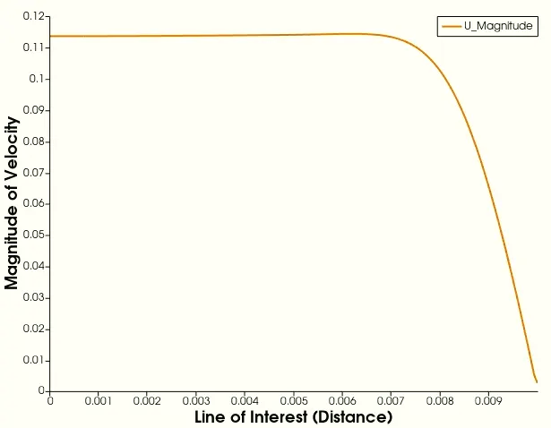
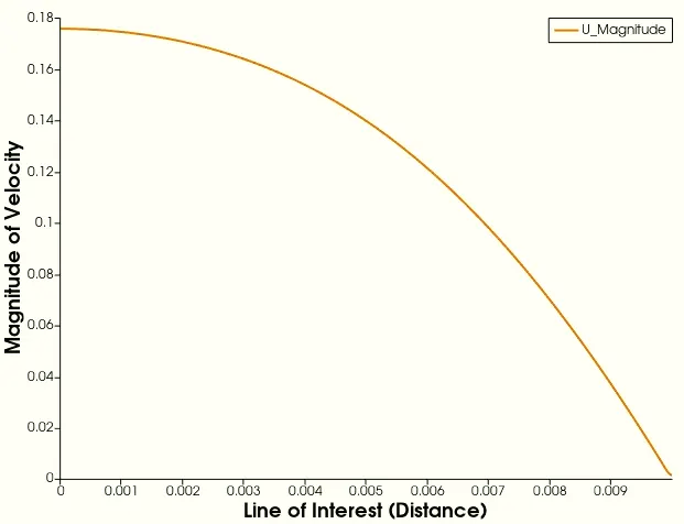
The velocity plot at 0.05 m from the inlet face is:-
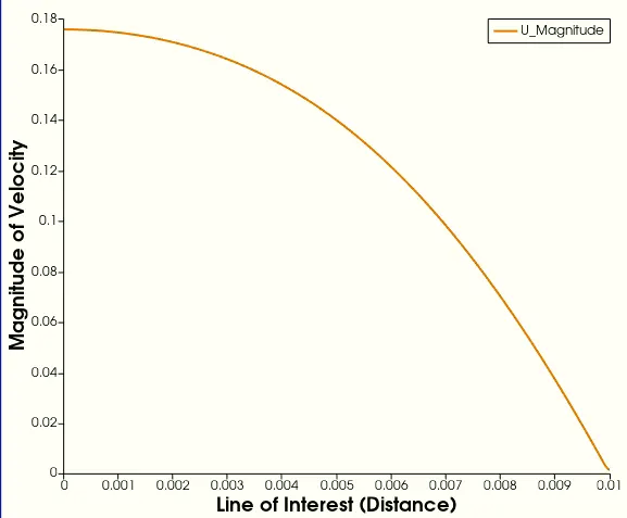
The velocity plot at 2.52 m from the inlet face is:-
The velocity plot at 3 m from the inlet face is:-
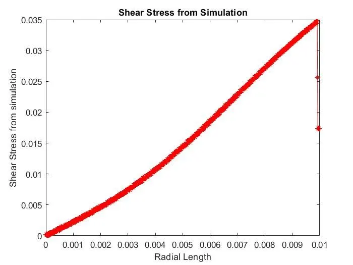
Shear Stress calculated from the simulated results is :-
Conclusions:-
It is clearly evident from the plot that beyond theoretically calculated hydrodynamic length, the velocity curve experience little to no change.
Also there is a little variation in the maximum velocity calculated analytically and by simulation. This error may be attributed to the numerical error.
The analytically fully developed flow is very similar to that of the simulated flow.
The maximum velocity is slightly diminished in the case of simulated flow. The order of error can be attributed to the numerical error in simulation.