Week 11: Project 2 - Emission characterization on a CAT3410 engine

Aim:

• To run the simulation of two type of piston bowl and characterize the emission(soot, Nox, UHC).

1. W-type piston / Open W piston
2. Omega piston / Re-entrant piston

• Create cut-plan animations showing Soot, Nox and UHC and compare them between the omega and the open-w pistons. 
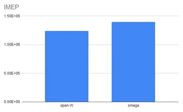
• Compare the imep and power values graphically.

Introduction

Diesel engine is widely used for non-road purposes, as well as transportation purposes because of its thermal efficiency, reliability and fuel economy. Diesel engine technology with higher efficiency and lower emission is still being developed. These developments up to now have led to an increase in the interest in the diesel engines for agriculture and maritime sectors where fuel economy is an important parameter. The numerical realization of a mathematical model for a physical system, in the form of a computer program, is shaped by a combination of practical and philosophical decisions which determine its ultimate form. A mathematical modeling of the internal combustion engine has been constructed and implemented as a computer program suitable for use on large digital computer system. The model strikes a balance between three competing factors: (1) the desire for physical realism, (2) the extent of experimental information on the physical processes occurring in the engine , and (3) the capabilities of today’s generation of computers. Modeling is a very useful approach for the development of internal combustion engine and optimization of its design parameters. Modeling of an internal combustion engine will develop as our understanding and knowledge of the physics  and chemistry mechanism of the phenomena and as computers continue to increase their ability to solve complex equations. The models describe the thermodynamics, fluid flow, heat transfer, combustion and emission formation events of the engines.

Combustion has been a key technology for transportation since the last century. Despite its central role in improving living standards, it has had significant adverse environmental impacts. Notably, the CO2 emissions it produces have contributed greatly to global warming. In addition, combustion creates noise and produces pollutants that reduce air quality in urban areas. Consequently, legislature around the world are introducing increasingly strict regulations requiring the automotive sector to reduce its emissions. For instance, the European Union has implemented legislation limiting the fleet average CO₂ emissions of vehicles to 130 g/km(depending on vehicle weight). Emissions of 130g CO₂/km correspond to a fuel consumption of around 5.6 liters per 100 km (5.6l/100 km) of petrol or 4.9 l/100 km of diesel. This limit is expected to be reduced to 95 g/km in 2021 and then to between 68 and 78 g/km in 2025. Similar regulations have been or will be implemented in other countries. To meet these requirements, vehicle manufacturers are exploring a range of strategies to reduce emissions, including geometrical improvements, advanced combustion modes, turbo-charging, and variable valve timing. However, these techniques increase the complexity of vehicle engines and typically offer only marginal benefits.

The fuel used by IC engines also has major impact on our global environment. Burning of 1 kg of fuel consumes about 15 kg of air, and significant energy is required to pump it into and out of the engine. In addition, about 3kg of is generated, which contributes to the world’s annual production of 37 billion tons of , a major greenhouse gas (GHG). Some fear that GHGs can cause climate change with unpredictable consequences. To address this problem, the international Energy Agency’s roadmap is to reduce fuel use by 30-50% in new road vehicles worldwide by 2030, and in all vehicle by 2050. Although 2050 appears distant, the time required to bring new engines to production, together with the years needed for new technology to permeate the vehicle fleet, means that major effort will be required.

An alternative approach would be to replace emission-generating internal combustion engines with battery electric power-trains, which emit no harmful pollutants directly. This could be a viable solution if the electricity used to power the vehicles was generated from renewable sources. However, the capacity and working lifespan of currently available batteries are very limited, and the environmental friendly disposal of used batteries is challenging. Therefore, the complete replacement of internal combustion engines with battery electric power-trains is not currently a promising general solution to the environmental problems associated with transportation.

The grand challenge faced by engine and researchers over the next decades will be to devise technological advances that maximize the engine efficiency, minimize pollutant emissions, and optimize tolerance to a wide variety of fuels in power generation and transportation systems. Much recent engine research has focused on improving the understanding the ignition, which is highly dependent on the fuel’s chemical composition, and also on increasing the quality of the air-fuel mixture for improved combustion efficiency. Future legislation requirements for fuel consumption and emissions have prompted efforts to develop new engine technologies. This has resulted in extensive research on internal combustion engine systems because of their potential to

reduce fuel consumption and exhaust emissions. Two major factors controlling fuel/air mixing in ICE are the fuel injection system and the nozzle geometry. The present injection system needs to provide an improved spray characteristics such as spray penetration length, fuel atomization, droplet sizes and droplet size distribution to enhance a combustion system efficiency. Spray characteristics have a huge influence on the combustion system efficiency because the spray directly controls the dynamics of the combustion process. Spray dynamic are complex multi-scale physical phenomena that are highly sensitive to the injector nozzle geometry(cavitation), nozzle exit conditions(turbulence), and fuel injection pressure. These conditions can change the atomization behavior and course of physical processes of the spray after the nozzle exit. The measurement techniques have some limitations to incorporate all the physical processes. Also, it is very challenging to isolate all the physical processes. On the other hand, Computational fluid dynamics (CFD) simulations offer an alternative way of studying these processes, and are becoming an increasingly reliable and effective tools for studying phenomena such as spray injection and its subsequent development. On the other hand, the simulation techniques are becoming an increasingly reliable and effective tool for the detailed study of insight phenomena including spray injection and its subsequent processes. However, due to different scales are involved to address the atomization and nozzle flow, it is challenging the entire phenomenon (atomization and nozzle flow) in the single CFD frame work.

At present, direct numerical simulations (DNS) is the only computational method capable of resolving all length scales involved in the atomization processes [5]. Unfortunately, its high computational cost largely restricts its use to academic test cases. An alternative method with lesser computational costs, the large-eddy simulation (LES) technique, has been widely used to simulate unsteady multiphase phenomena. LES can accurately capture intrinsically time- and space-dependent phenomena because it directly resolves large-scale turbulent structures and uses a model to describe sub-grid scale structures.

Spray modeling

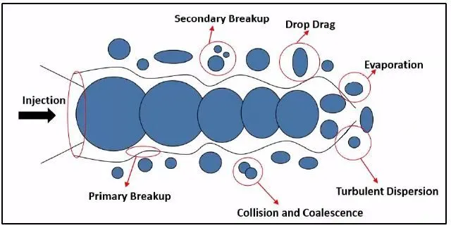
Spray models are very important in engine CFD simulations because they influence the subsequent mixing, ignition, combustion and emission predictions. Spray models include those describing the flows inside injector nozzles, atomization of the continuous liquid after the fuel leaves the injector nozzle (primary breakup model), breakup of the formed liquid drops (secondary breakup model), momentum exchange between the liquid and gas phases (i.e., the drag force that liquid droplets experience and the deformation of the droplets), collision between liquid drops and its possible outcomes (collision model), interaction between sprays and walls (e.g., wall-film model), and evaporation of the liquid fuel (evaporation model).

Spray sub-models

Various sub-models were implemented to account for the effects of turbulence , coalescence , evaporation , and droplet breakup in the fuel spray simulation. A spray process can be represented in the following diagram.

Discrete phase modeling

Fluent provides a model that is especially for spray simulations, or more general suspended particle trajectory simulations. This is the Discrete Phase Model (DPM) and it is based on the so-called Euler-Lagrange method. In the computational domain there are two separate phases present, namely, the continuous and the discrete phase (particles). The transport equations are solved for the continuous phase only and the motion of particles is dealt with particle trajectory calculations. Through an iterative solution procedure, the mass, momentum and energy interaction between both phases can be realized.

Combustion Modeling

Various combustion models have been developed to simulate a wide variety of combustion phenomena in both spark-ignited (SI) and compression (CI) engines, including spark and auto ignition, laminar and turbulent combustion, premixed, non-premixed and stratified-charge combustion, kinetics and mixing-controlled combustion, and flame propagation combustion. For CI engines, combustion modeling also must resolve two steps: low-temperature chemistry which leads to auto ignition, and the following high-temperature reactions which contribute most of the heat release.

Since combustion in DI engines is turbulent and many turbulent combustion models with different levels of complexity have been proposed for engines applications, including models based on RANS and LES turbulence models. However, since RANS models, specifically the k- model and its variants, are the most commonly used turbulence models at present. In general, there are two ways to describe the combustion process in engine cylinders. One is to use a combustion sub-model to describe the overall combustion characteristics (i.e., flame propagation, reaction rates, and so on) of a combustion process. Combustion models such as mixing-controlled combustion models, flamelet models, and probability density function (PDF) models belong to this category. The other way is to use a detailed reaction mechanism which describes the complex reaction pathways and reaction rates of the important chemical reactions involved in the combustion process and solve for the rate of change of each species in the mechanism.

Before describing the models, two variables which are used in these models are introduced. The first is the mixture fraction (Z) and the second is the reaction progress variable (c). The mixture fraction quantifies the local mass fraction of materials that originate from the reactant fuel. It is mostly used in the analysis and modeling of non-premixed reacting systems. For premixed combustion systems, a reaction progress variable is used. The progress variable increases from zero in the unburned reactants to unity in the burned products. The calculation of the progress variable can be associated with either the mass fraction of a specific species (combustion products) or temperature.

CONVERGE offers two different methods for modeling the ignition and combustion processes. The first method uses separate models for ignition and combustion. These models
are based on the Shell ignition model and the Characteristic Time Combustion model, and this method is relatively computationally inexpensive. The second approach, described in the SAGE detailed chemical kinetics solver section, considers much of the chemistry taking place in combustion applications. Although the runtime using detailed chemistry can be significantly longer than with the first approach, the accuracy of the simulation may be greatly enhanced with the inclusion of detailed chemistry. Nonetheless, there is still often a need for the rapid turnaround time that can be achieved when the simpler models are used. 

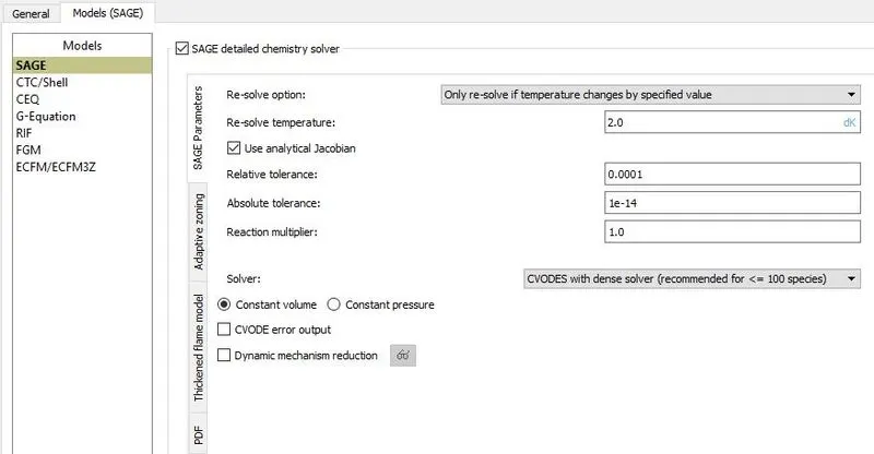
CONVERGE contains the SAGE detailed chemical kinetics solver which models detailed chemical kinetics via a set of CHEMKIN-formatted input files. To solve the systems of ordinary differential equations (ODEs), SAGE uses the CVODE solver, which is part of the SUNDIALS (SUite of Nonlinear and DIfferential/ALgebraic equation Solvers) package.

A chemical reaction mechanism is a set of elementary reactions that describe an overall chemical reaction. The combustion of different fuels can be modeled by changing the mechanism (e.g., there are mechanisms for isooctane, gasoline, n-heptane, natural gas, etc.). SAGE calculates the reaction rates for each elementary reaction while the CFD solver solves the transport equations. Given an accurate mechanism, SAGE (in addition to AMR) can be used for modeling many combustion regimes (ignition, premixed, mixing-controlled). You can use SAGE to model either constant-volume or constant-pressure combustion. Note that SAGE consistently uses CGS units for all calculations.

Geometry preparation:

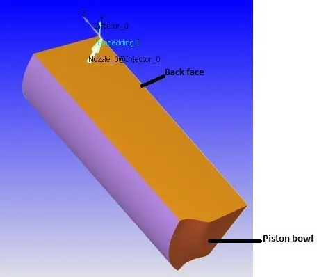
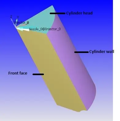
Open-W piston Geometry

          

Omega Piston Geometry

    

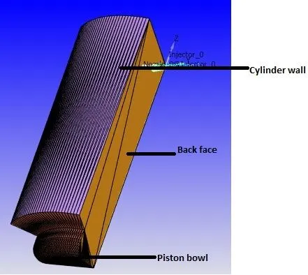
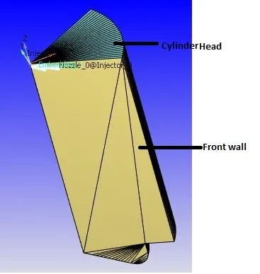
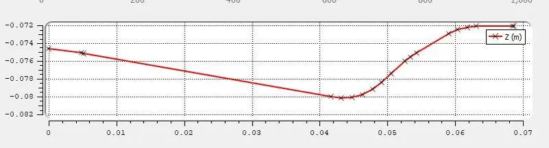
A sector of 60 degree of engine volume is used for geometry. The following piston bowl profiles are imported along with the geometric details of cylinder to create this engine sector.

Omega piston

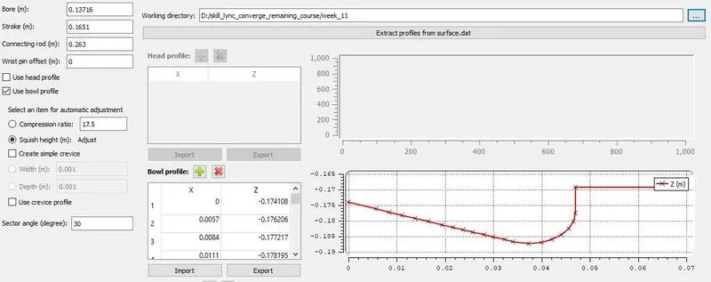
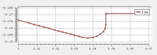
Open-W piston

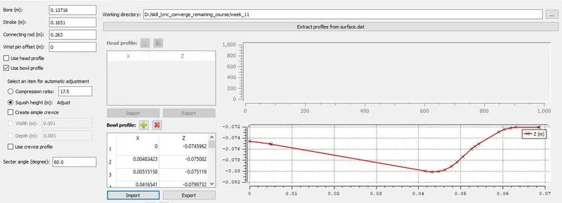
Sector angle

It is calculated as we have assume 6 nozzles inside the injector.

Sector angle =  `frac{360^@}{Nos. of Nozzles}`= `60^@`

Note:

Before processing for case-setup, we check the diagnosis to make sure that geometry is free from errors.

 Case setup

Open the case setup

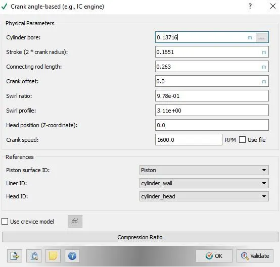
Physical parameters

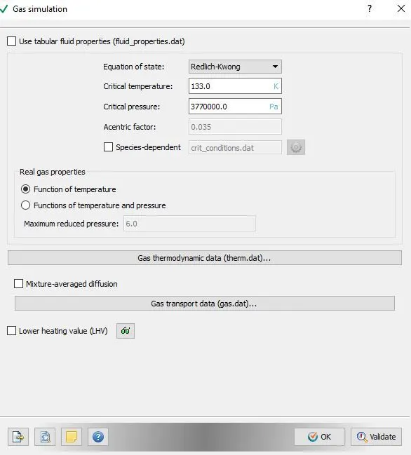
Materials

   

  

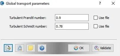
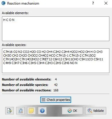
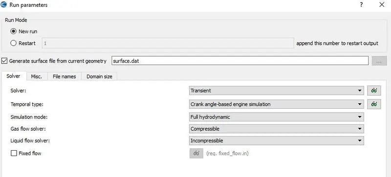
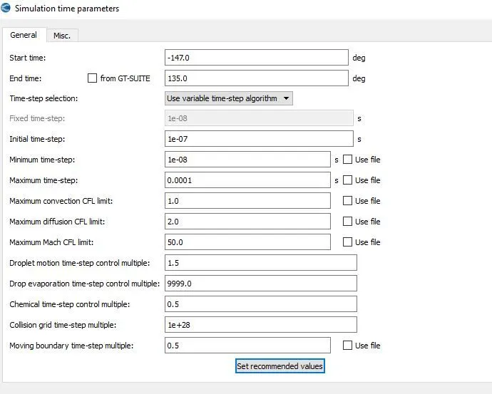
Simulation parameters

     

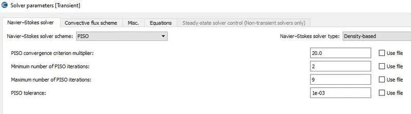
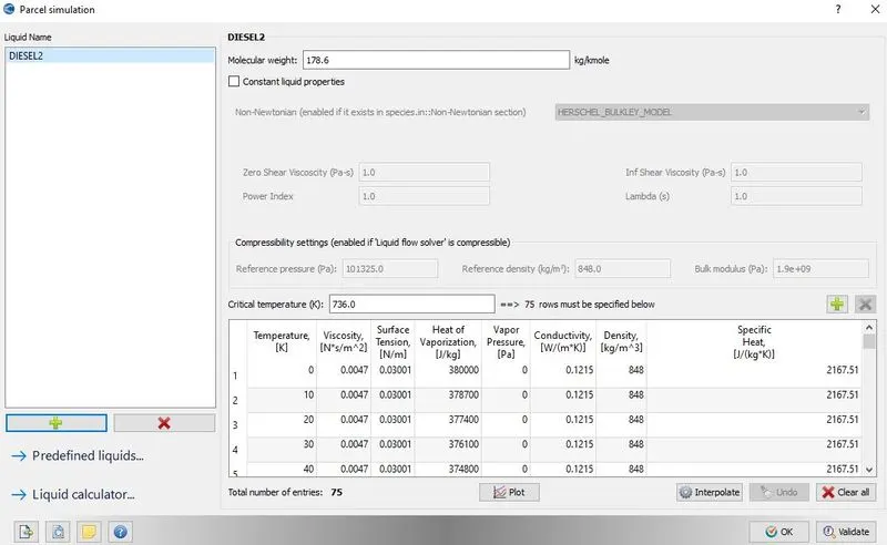
Parcel simulation

In this case we are using the C7H16(n-heptane) as our fuel spray.

Boundary Conditions:

Region Name	Boundary Name	Boundary type	Boundary Motion	Temperature	Motion details	Region initial pressure	Region initial temperature	Region initial species
Cylinder region	Piston	Wall	Moving	553	Piston motion	197000	355	CO2: 0.0014304 H2O: 0.0006296 N2: 0.76795 O2: 0.23029
	Front face		Periodic	-	60 degree rotation about z
	Back face		Periodic	-	Matching boundary
			Stationary	433
	Cylinder wall
	Cylinder head		Stationary	523

Mesh

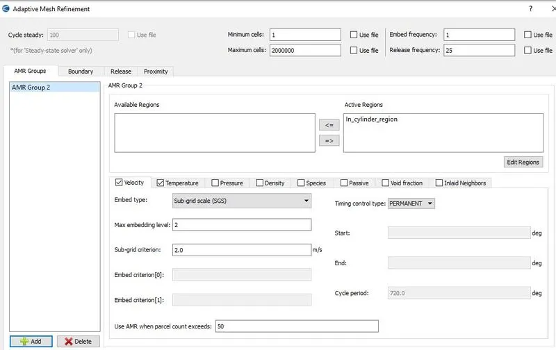
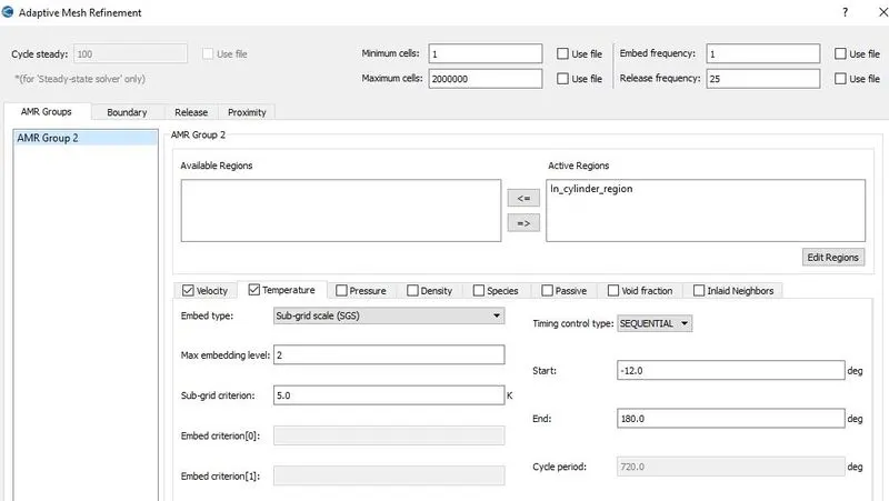
A base mesh was created with element size of 1.4mm and following embedding and AMR settings were applied to refine the mesh as required.

Sr No.	Embedding name	Embedding type	Embedding on	Embedding mode	Scale`rightarrow`Element size	Embed layers	Radius 1 at co-ordinate 1	Radius 2 at co-ordinate 2	Cylic details
1	Piston embedding	Boundary	Piston	Cyclic	1`rightarrow`0.7mm	1	-	-	From -20 deg to 180 deg(720 deg period)
2	Cyl head embedding	Boundary	Cylinder head	Cyclic	1`rightarrow`0.7mm	1	-	-	From -20 deg to 180 deg(720 deg period)
3	Nozzle	Nozzle	Volume	Cyclic	2`rightarrow`0.35	-	Radius = 0.001m and 0.003m Length= 0.01m		From -12 deg to 15 deg(720 deg period)
				Base mesh or scale 0 mesh element size is 1.4mm

Velocity AMR

Temperature AMR 

Spray modeling:

In the general tab we do the following setting.

• Parcel distribution: we choose the option cluster parcels near cone center.
• Turbulent dispersion : we choose the O'Rourke model.
• Droplet evaporation : We choose the Frossling model.
• Evaporation Source: We choose the option source specified species and choose C7H16.
• In the spray penetration tab, we choose the 0.97 for the liquid fuel mass fraction.
• Bin size for vapor penetrtion = 0.001
• Fuel mass fraction for calculating vapor penetration = 0.001
• Mass diffusivity constant: We use the Diesel default values.

In the collision/Breakup/Drag, we do the following settings.

• Collision model: Choose the NTC-collision model
• Collision outcomes: Post collision outcomes
• Level of collision mesh : 2
• Drop drag model: Dynamic drop drag model

In the wall interaction , we do the following settings.

• Spray wall interaction model: Rebound/slide

In the injectors tab, we do the following settings.

• Injected species: Diesel2
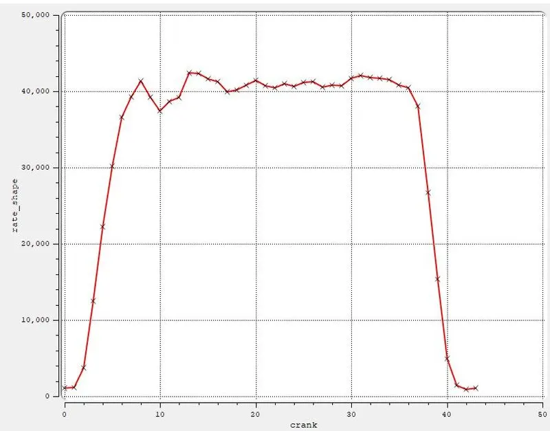
• Rate shape : profile as shown in the below figure.

• Models: Kelvin Helmolthz model
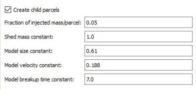
• Child parcels: 

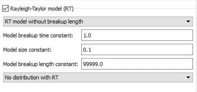
• Rayleigh Taylor Model

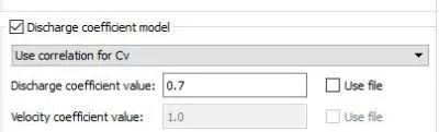
• Discharge coefficients

• In the Mass,time and temperature we do the following settings.

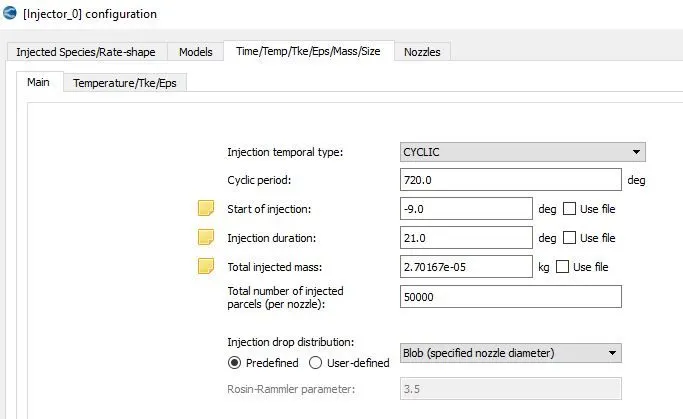
Nozzle_0 configuration

   

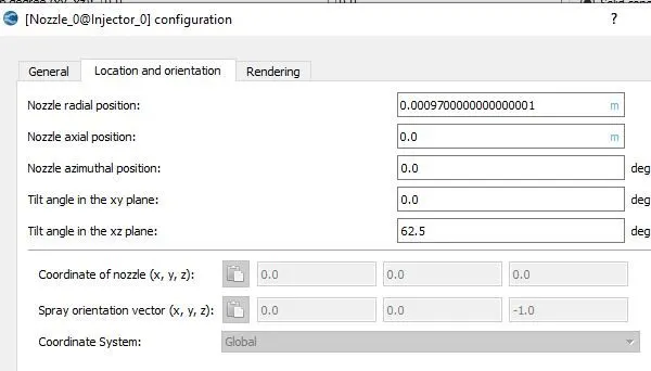
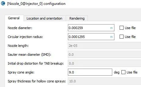
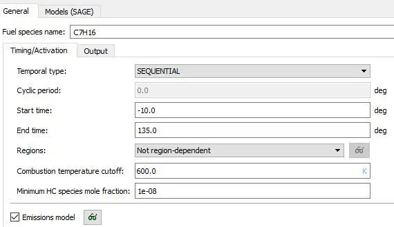
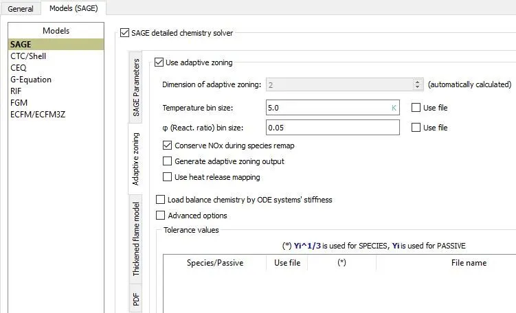
Combustion Modeling

  

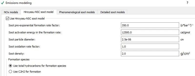
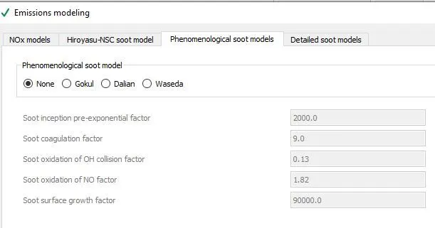
Emissions modeling

     

    

Results:

Pressure

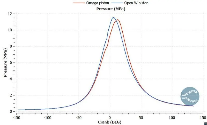
Behaviour of the pressure plot is correct for both pistons. In the above figure we can easily see that the open-W piston has the highest pressure than the omega piston.

Mean temperature

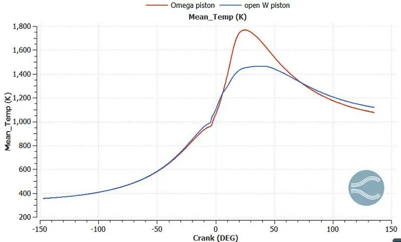
In the above graph, we can easily observe that the mean temperature is higher in omega piston as compared to the open-W case. This higher mean temperature produces the faster burning of fuel. This higher temperature is going to rise the NOx and soot formation.

        

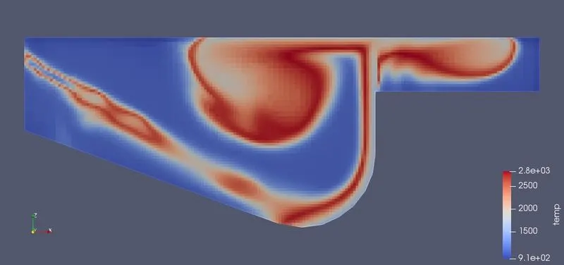
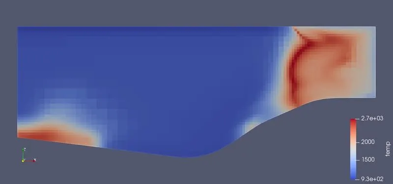
In the contours images, we can easily observe the temp variations in the omega and open-W piston.

Max temperature

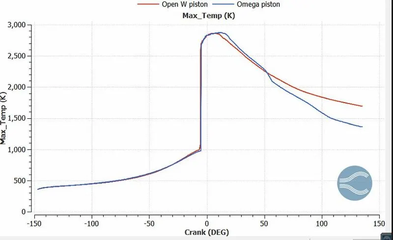
Max temperature in both cases (Omega and open-W) are almost equal.

Heat release rate

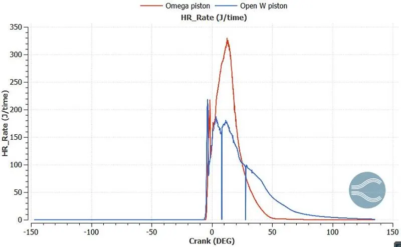
The heat release rate can be shown in the above figure. We can easily observe that Omega piston has a higher heat release rate than the open-W piston. The faster burning in the case of omega piston is the reason of higher heat release rate.

Integrated Heat release rate

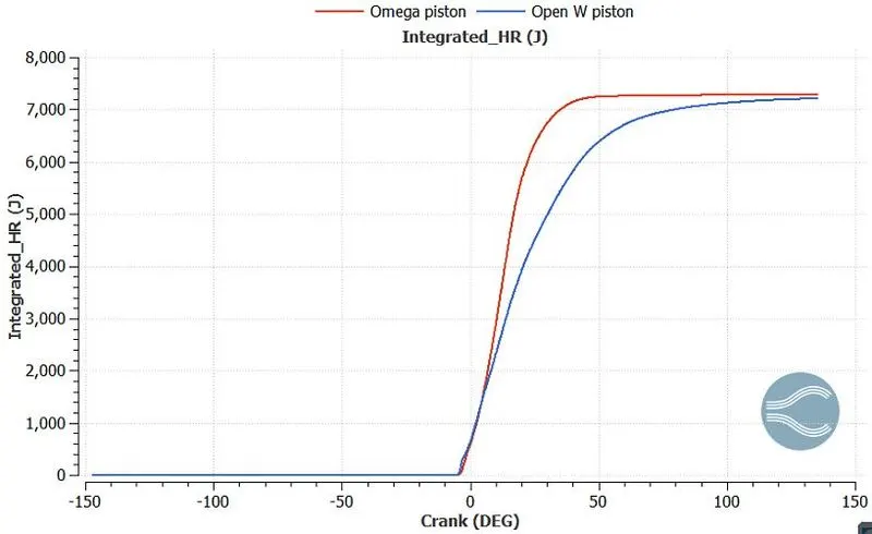
In the above plot we can easily see that omega piston has the higher integrated_HR, this is happening due to high temperature in omega piston.

Spray parcels

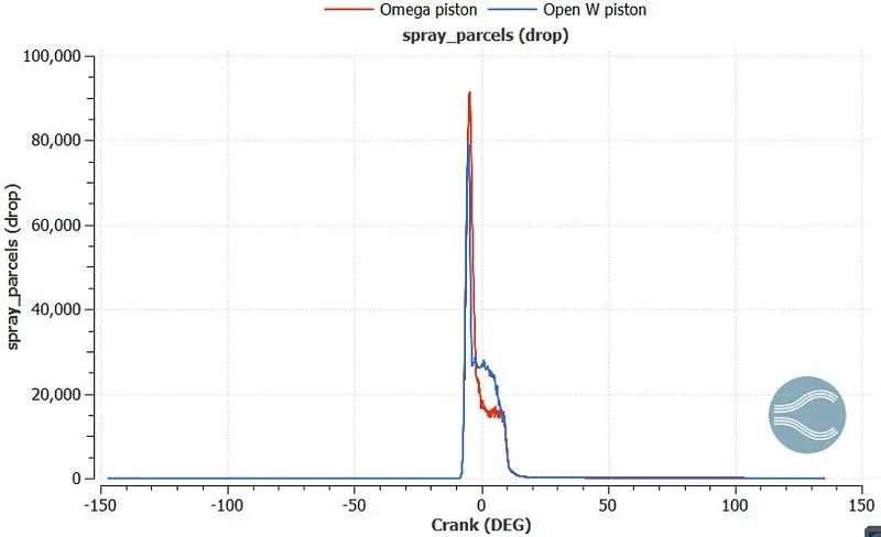
The above plot shows the no of parcel in the chamber which are in the form of droplets. In open-W case, curve has a lower peak because when the spray enter into the chamber it travels for some distance and then it forms a film on the piston surface. The fuel film eventually burns out by evaporation but it reduces the number of parcels in drop phase. But in Omega case,  the parcels gets enough time to evaporate and thus they burn out faster and we can see less drop parcels after 10 degree crank angle.

Spray penetration

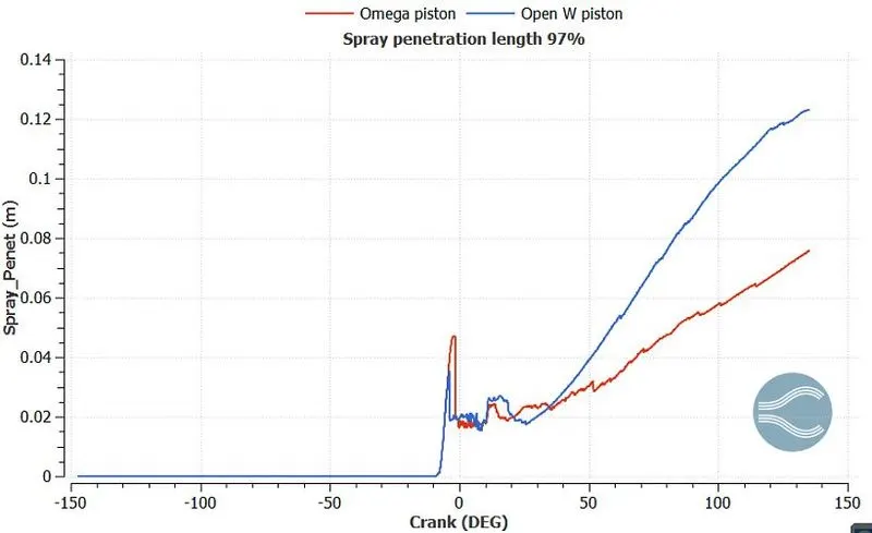
Spray penetration length was defined as the distance from the nozzle tip to the farthest spray region from the nozzle tip. In the above plot we can easily see that the open-W piston have long penetration than the Omega piston. The reason behnid the increase of penetration length in Open-W piston is that due to low temperature droplets are not disintegrated faster abd that's why do not evaporate faster. While in Omega piston case, due to instant increase in temperature droplets are evaporated faster.

Unburned hydrocarbon

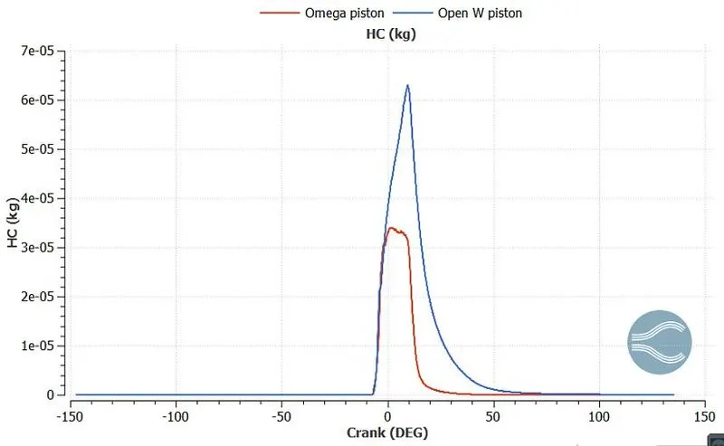
In the above hydrocarbon plot we can easily see that the open-W piston has a high hydrocarbon than the omega piston. The reason behnid of low hydrocarbon in omega piston is that due tp high temperature fuel evaporated fastely and there is not adequate amount of fuel is remaining. But in the case of open-W piston, we can observe in the above plots thers is not any kind of increase in temperature is occuring, that's why fuel is not completely burn and there is adequate amount of fuel is remaing which produces hydrocarbons.

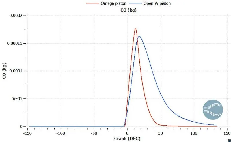
In the CO plot, we can easily see that the omega piston has the highest peak then of open-w piston. But in this case we are not considering the peaks, we can see that the area under curve in open-W case has more than the omega piston. More area occupy means that there is too much amount of carbon monoxide.

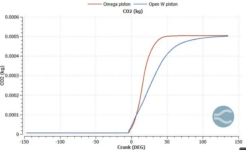
Combustion occuring in omega piston case is fastly

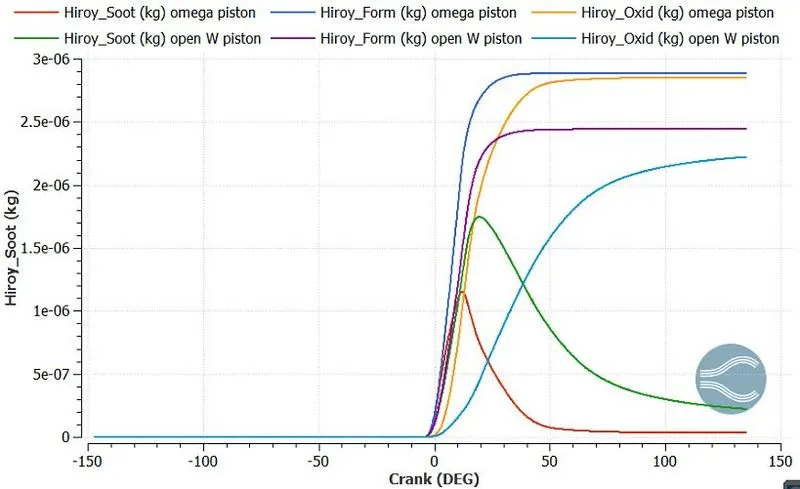
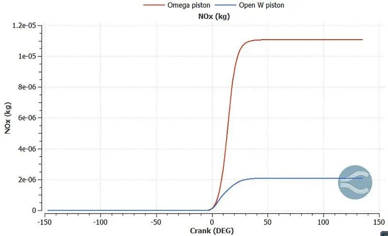
Due to high temp in omega piston case, NOx are produces and due to low temperature in open-W piston NOx are not produces. NOx always produces at high temperature because at high temperature all the fuel are burn, only the amount of air is remaining that's why NOx are produces.

Combustion Efficiency

Open W bowl piston `eta_c = frac{IHR}{m times LCV_(fuel)` Where IHR is the integrated heat release rate and we obtained from the IHR graph. LCV is the lower calorific value IHR = 7206.21 LCV for diesel = 45.5 MJ/kg m = 1.621e-4 kg 97.7040%

Omega bowl piston eta_c = frac{IHR}{m times LCV_(fuel) Where IHR is the integrated heat release rate and we obtained from the IHR graph. LCV is the lower calorific value IHR = 7279.44 LCV for diesel = 45.5 MJ/kg m =1.621e-4 kg 98.6969%

 Power and torque calculation

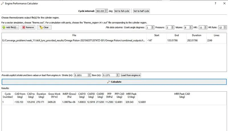
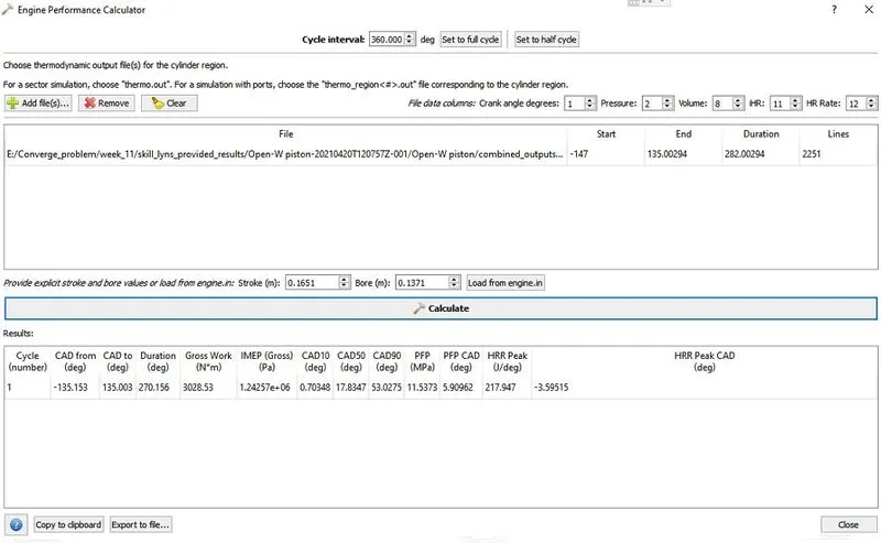
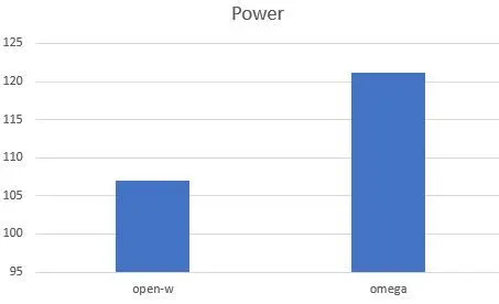
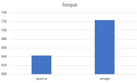
The result of engine performance is calculated from tool of Converge CFD. It gave the following output Parameter Open W Omega Gross work(Nm) 3028.53 3409.28 Duration used to calculate gross work (deg) 270.156 270.171 IMEP(Pa) 1.24076e+6 1.39575e+6 CA 10 (deg) 0.70348 1.00833 CA 50 (deg) 17.8347 12.5019 CA 90 (deg) 53.0275 27.5283 Power calculation for Omega piston using engine calculator Work = 3409 Duration = 270.171 Power =work/sec RPM = 1600 RPS = 26.667 1 rotation = 360 degree DPS = 26.667*360 = 9600 Time(sec) = 270.171/9600 = 0.0281428 Power = 3409/0.0281428 = 121132.2256 KJ,     121.1322256 KW Torque calculation Power = 2*pi*N*T Torque(T) = Power/(2*Pi*N) Where N- rev/sec              T-Torque (N.m)              Power – KW             N = 26.667 rev/s Power = 121132.2256 KJ,     121.1322256 KW Torque = 723.312369 Power calculation for Open-W piston using engine calculator Work = 3028 Duration = 270.171 Power =work/sec RPM = 1600 RPS = 26.667 1 rotation = 360 degree DPS = 26.667*360 = 9600 Time(sec) = 270.171/9600 = 0.0281428 Power = 3028/0.0281428 = 107,594.12709 KJ,      107.594KW Torque calculation Power = 2*pi*N*T Torque(T) = Power/(2*Pi*N) Where N- rev/sec              T-Torque (N.m)              Power – KW             N = 26.667 rev/s Power = 107,594.12709 KJ,      107.594KW Torque = 642.472823

Conclusion table

Sr.No	Type	Type of parameter	Open W	Omega
1.	Thermodynmic	Maximum temperature(k)	2860.67	2867.53
		Maximum Mean temperature(k)	1462.79	1768.26
		Maximum Pressure(bar)	10.5628	11.2539
		Maximum HRR(J/s)	318.589	178.122
		IHR(J)	7206.21	7279.44
2.	Spray	Maximum spray penetration length(m)	0.0121596	0.0739
		Maximum parcels in drop phase	78361.8	91535
3.	Emissions at the end of stroke(kg)	CO2	0.000500331	0.00050501
		CO	0.000162476	0.000176188
		Unburned HC	6.28216e-08	3.31221e-05
		NOx	2.08841e-06	1.10645e-05
		soot	1.74671e-06	1.15002e-06
4.	Performance parameters	Combustion efficiency	97.7040%	98.6969%
		Gross work (Nm)	3028.53	3409.28
		Torque (Nm)	642.472823	723.312369
		Power (KW)	107.594	121.1322256
		IMEP (pa)	1.24076e+6	1.39575e+6
		CA 10 (deg)	0.70348	1.00833
		CA 50 (deg)	17.8347	12.5019
		CA 90 (deg)	53.0275	27.5283

Omega Piston Velocity AMR

Omega Piston Temperature AMR 

Open-W Piston Velocity AMR

Open-W Piston temperature AMR

Results discussion

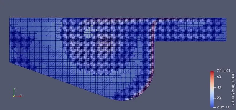
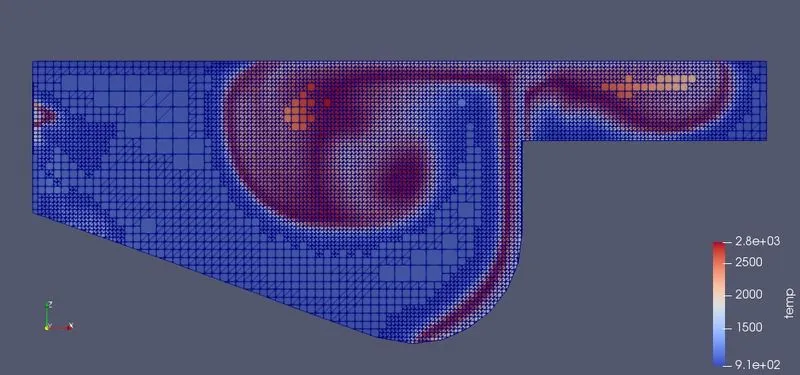
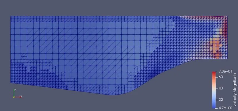
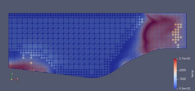
In the above figure, we can see the velocity and temperature AMR of Omega and Open-W piston. A sudden rise in the cells can be seen as the spray injection start. Omega piston had more cells because there was a more volume compared to open-W case.

Animation videos of Omega piston

Spray animation of Omega piston

Hiroy soot animation of Omega piston

NOx animation of Omega piston

CO animation of Omega piston

CO2 animation of Omega piston

H2 animation of Omega piston

H2O animation of Omega piston

O2 animation of Omega piston

Animation videos of Open-W piston

Spray animation of Open-W piston

Hiroy soot animation of Open-W piston

NOx animation of Open-W piston

CO animation of Open-W piston

CO2 animation of Open-W piston

H2 animation of Open-W piston

H2O animation of Open-W piston

O2 animation of Open-W piston

Conclusion

• In this challenge, we run the simulation of Omega and open-W piston.
• Every design of piston have their own advantages and disadvantages.
• In the omega piston design, unburned hydrocarbon are produces but in the open-W piston case rate of production of NOx are high.
• If we compare the both designs of piston then in comparison omega piston design is batter than the open-W piston.