Week-11 Challenge: Braking

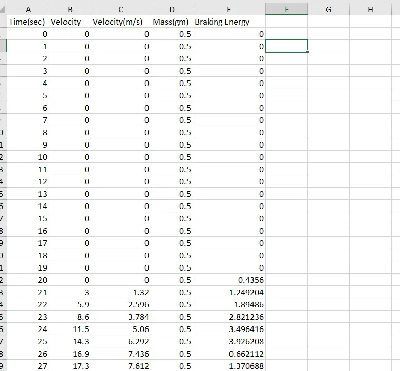
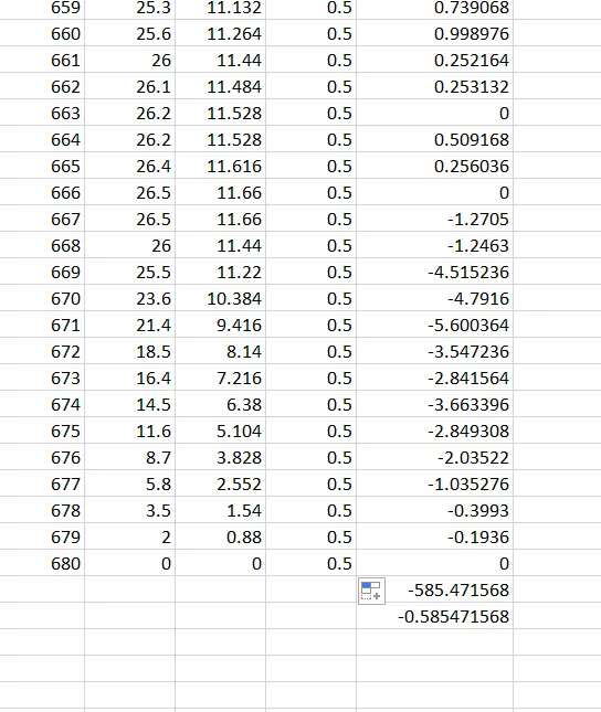
1) Braking Energy = (1/2)*m*v^2

 Where, Braking Energy is the kinetic energy in unit of Joule.

 m= Total Mass of the Vehicle (Vehicle Mass + Pay Load) in unit of Kg.

 v= (Initial Velocity-final Velocity) in unit m/s.

UDDS drive cycle is considered and for 11 mins approximately 0.5 kJ energy is required for braking since it a urban driving. The result have been attached in excel below.

 

2) The elecric motor cannot develop braking torque at high spped similar to starting. Peak Acceleration Torque and Peak Deceleration torque are not equal for Electric Vehicle Motor. So the Peak Torque during acceleration and the Peak torque during deceleration or braking are not equal. Acceleration is usually higher, at low speed we get higher Torque but high speed the value of the torque gets lower.

So for example. we cannot say that the motor which is producing 5Nm Torque for Acceleration can also produce -5Nm of Braking Torque. So beacuse we operating the Motor in Field Weakening region or we are operating the Motor above base speed we must know that the torque is compromised or the torque value is lower. So Electric motor can’t develop braking torque at high speed similar to starting, because Braking Torque of an EV Motor is not as high as the Acceleration Torque.  

There are 2 types of brake control strategies in which the electrical and mechanical brakes are coordinated. These are as follows:

Series Brake control - In this method the mechanical brake and regenrative barkes are applied one after the other.

Parallel Brake control -  In this method the mechanical brake and regenrative barkes are applied simultaneously.

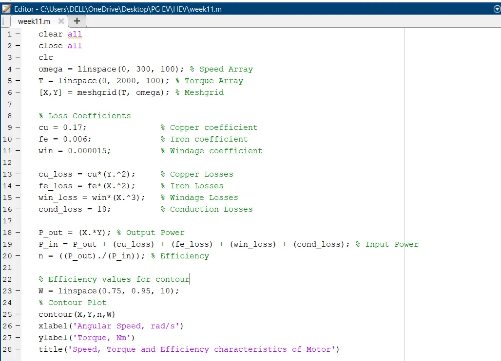
3) A MATLAB program which plots contour of given motor speed, torque and efficiency values is as follows:

The obtained plot for the above m.code is as follows:

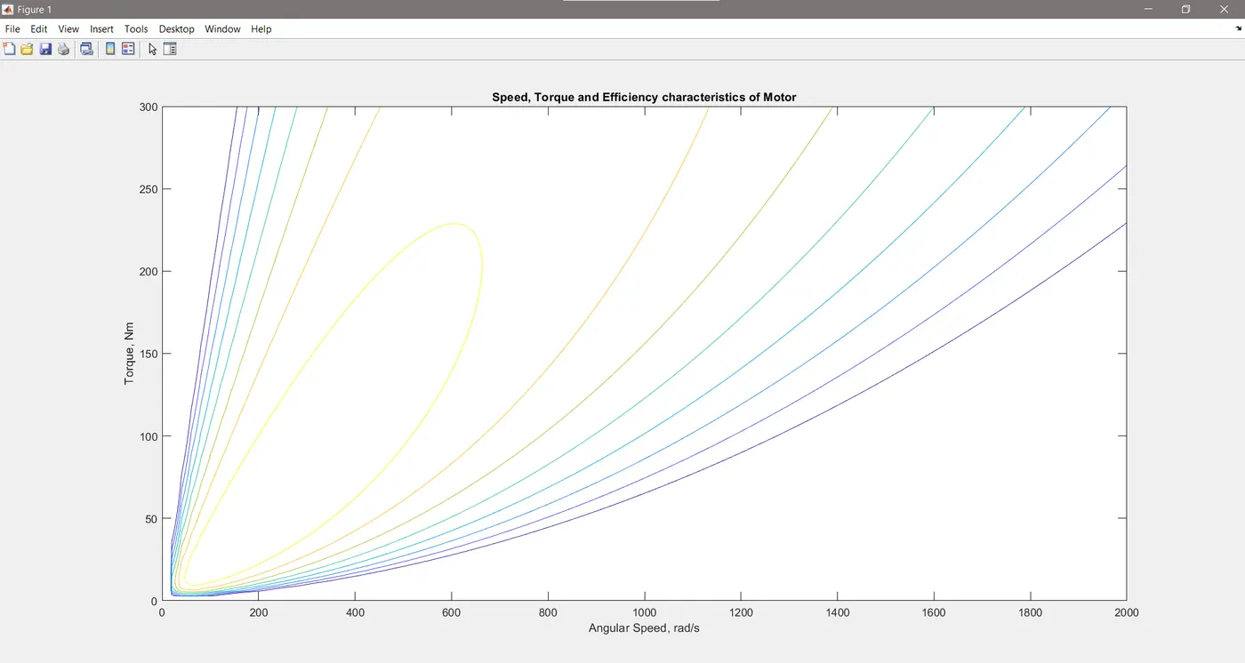
In this MATLAB script, the arrays for the speed and the torque of the motor using the ‘linspace’ command is created. For the speed, consider a range of values from 0 to 300 radians per second whereas for the torque, consider a range of values from 0 to 2000 Nm.These arrays are then used to create 2D grid coordinates using the ‘meshgrid’ command. These coordinates will help in the creation of the contour plot. In order to find the efficiency of the motor, we need to consider the various losses that occur in the motor’s operation. These are copper losses, Iron losses, Windage losses and Conduction losses.

These various losses are dependent on the speed and the torque of the motor. They each also have a characteristic constant of proportionality which are all assumed for the following calculations and represented as 'K'. In each calculation, the speed and the torque are represented respectively as ω and T. The values of coefficients are taken as general values. Conduction losses are assumed to be 18 Joules.

Finally we plot the contour with the 'contour' command. In addition, an array for the efficiency values we want to plot for is created called 'W' and is assigned for values ranging from an efficiency level of 0.75 to 0.95. This array is used in the creation of the contour. Axis labels and a title is also made for better readability.