Week-11 Challenge: Braking

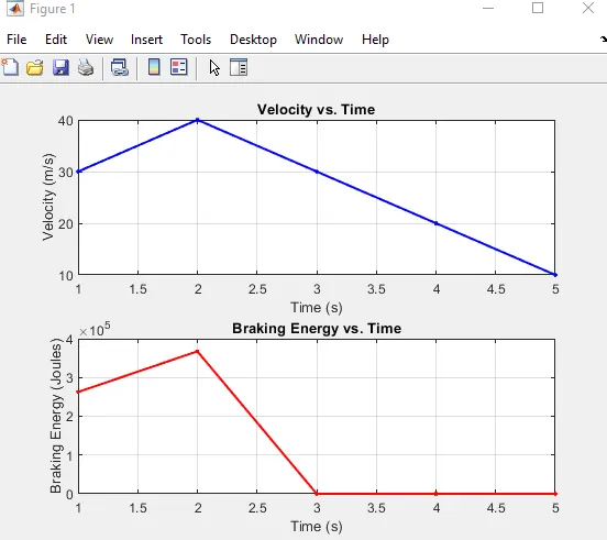
1.For a defined driving cycle, calculate the energy required for braking.

ANS:

Braking:

The function of the braking system is to retard the speed of the moving vehicle or bring it to rest in the shortest possible distance whenever required. The vehicle can be held on an inclined surface against the pull of gravity by the application of a brake. Brakes are mechanical devices for increasing the frictional resistance that retards the turning motion of the vehicle wheels. It absorbs either kinetic energy or potential energy or both while remaining in action and this absorbed energy appears in the form of heat. While moving down a steep gradient the vehicle is controlled by the application of brakes. In this case, brakes remain in action for a longer period making it imperative to dissipate the braking heat to the atmosphere as rapidly as possible.
Automobiles are fitted with two brakes; the service or foot brake and the emer­gency or hand brake. The foot brake is used to control the speed of the vehicle and to stop it, when and where desired, by the application of force on the brake pedal. The hand brake, applied by a lever, is used to keep the vehicle from moving when parked. Hand brakes are called emergency brakes because they are applied when the service brake fails. Virtually all vehicles are now equipment with 4-wheel brakes. The front brakes must operate without interfering with the steering action.
The brakes must be capable of decelerating a vehicle at a faster rate than the engine is able to accelerate it. Normally brakes have to absorb three times the amount of engine horsepower energy in its equivalent form.

to calculate the braking enery we have to create a excel sheet of driving cycle:

now we will use a matlab code for generating the brake energy:

fine the vehicle's mass (in kg)

mass = 1500; % Replace with your vehicle's mass

 

fine the time intervals and speed profile during the driving cycle

% You can modify this data based on your specific driving cycle.

time_intervals = [0, 1, 2, 3, 4, 5]; % Time intervals in seconds

speed_profile = [20, 30, 40, 30, 20, 10]; % Speed at each time interval in m/s

 

fine braking efficiency (η) as a value between 0 and 1

braking_efficiency = 0.7; % Replace with the actual efficiency

 

% Initialize variables to store total brake energy, time points, and braking energy

total_brake_energy = 0;

time_points = [];

braking_energy = [];

 

% Initialize variables for velocity vs. time plot, braking energy vs. time plot, and average brake energy

velocity = [];

time = [];

average_brake_energy = 0;

 

calculate kinetic energy and brake energy

for i = 2:length(time_intervals)

delta_t = time_intervals(i) - time_intervals(i - 1);

 

calculate kinetic energy at the start and end of the interval

KE_start = 0.5 * mass * speed_profile(i - 1)^2;

KE_end = 0.5 * mass * speed_profile(i)^2;

 

calculate the change in kinetic energy during this interval

delta_KE = KE_start - KE_end;

 

% Check if there was braking (negative change in kinetic energy)

if delta_KE < 0>

calculate and accumulate brake energy

brake_energy_i = -delta_KE * braking_efficiency;

total_brake_energy = total_brake_energy + brake_energy_i;

 

% Store time points and braking energy for the plot

time_points = [time_points, time_intervals(i)];

braking_energy = [braking_energy, brake_energy_i];

else

% For non-braking intervals, set braking energy to zero

time_points = [time_points, time_intervals(i)];

braking_energy = [braking_energy, 0];

end

 

% Store time points and velocity for the plot

time = [time, time_intervals(i)];

velocity = [velocity, speed_profile(i)];

end

 

calculate the average brake energy (total brake energy divided by the number of braking events)

num_braking_events = sum(braking_energy > 0);

if num_braking_events > 0

average_brake_energy = total_brake_energy / num_braking_events;

end

 

% Plot velocity vs. time

figure;

subplot(2, 1, 1);

plot(time, velocity, 'b.-', 'LineWidth', 1.5);

title('Velocity vs. Time');

xlabel('Time (s)');

ylabel('Velocity (m/s)');

grid on;

 

% Plot braking energy vs. time

subplot(2, 1, 2);

plot(time_points, braking_energy, 'r.-', 'LineWidth', 1.5);

title('Braking Energy vs. Time');

xlabel('Time (s)');

ylabel('Braking Energy (Joules)');

grid on;

 

% Display the total brake energy and average brake energy

fprintf('Total Brake Energy: %.2f Joules\n', total_brake_energy);

fprintf('Average Brake Energy: %.2f Joules per braking event\n', average_brake_energy);

 

we get the results in plot:

 

 

 

2.Why electric motor can’t develop braking torque at high speed similar to starting? How electric and mechanical brakes are coordinated?

 

ans:

 

1. Back Electromotive Force (Back EMF):

 

- **Back EMF** is a phenomenon that occurs in electric motors when they rotate. As the motor spins, it generates a voltage opposing the applied voltage. This opposing voltage limits the current flowing through the motor windings, which, in turn, limits the amount of torque the motor can produce. 

 

- At low speeds or during startup (when the motor is stationary), Back EMF is minimal, and the motor can produce its maximum starting torque. However, as the motor speeds up, Back EMF becomes more significant, reducing the net voltage across the windings and, consequently, the available torque.

 

2. Power Limitations:

 

- Electric motors have a maximum power output determined by their design and power supply. Power is the product of voltage and current (P = VI). At high speeds, the motor may reach its power limit because it's producing both mechanical power (torque * speed) and electrical power (voltage * current).

 

- Increasing the torque at high speeds would require more electrical power, which could exceed the motor's power rating or the capabilities of the power supply. Operating a motor beyond its power limits can lead to overheating, reduced efficiency, or damage.

 

3. Cooling and Thermal Considerations:

 

- High-speed operation generates more heat in the motor. Electric motors are designed with thermal limits to ensure they don't overheat. Running a motor at high torque and high speed can exceed its thermal capacity, potentially causing overheating or requiring additional cooling mechanisms.

 

Now, let's discuss the coordination of electric and mechanical brakes:

 

Regenerative Braking:

 

- Regenerative braking is an essential feature in many electric vehicles and systems. When the driver applies the brakes, the electric motor temporarily acts as a generator. It converts the vehicle's kinetic energy back into electrical energy, which can be stored in the battery or dissipated as heat through resistors.

 

- Regenerative braking is highly efficient and helps to extend the vehicle's range by recovering energy that would otherwise be wasted as heat in traditional friction brakes.

 

Mechanical Brakes:

 

- While regenerative braking can handle most of the braking needs, mechanical brakes are still essential. They serve as a backup and are used for scenarios where regenerative braking alone may not suffice, such as emergency stops, parking, and situations that exceed the motor's braking capacity.

 

Brake Control Systems:

 Modern vehicles use sophisticated brake control systems that manage the coordination between regenerative and mechanical braking. These systems ensure a smooth transition between regenerative and friction braking and optimize the balance between them based on various factors:

•   Vehicle Speed:At low speeds, regenerative braking is more effective. As speed increases, mechanical brakes may be engaged to provide additional stopping power.  
•   Battery State of Charge (SoC): Regenerative braking may be limited if the battery is already fully charged. In such cases, more reliance on mechanical brakes may be necessary.
•  Braking Force Required:The control system calculates the required deceleration and determines the appropriate combination of regenerative and mechanical braking to achieve it safely.

 

In summary, electric motors have limitations on braking torque at high speeds due to Back EMF, power constraints, and thermal considerations. Coordination between electric and mechanical brakes is managed by advanced control systems to optimize braking performance, energy efficiency, and safety in various driving conditions.

 

3.Make a MATLAB program which plots contour of given motor speed, torque and efficiency values. Attach the code as a .m file attach a screenshot of all the plots.

 

ans:

 

the  matlab code for the same is given :

 

define motor speed, torque, and efficiency data

speed = [1000, 2000, 3000, 4000, 5000]; % Speed in RPM

torque = [10, 20, 30, 40, 50]; % Torque in Nm

 

% Create a grid of speed and torque values

[speed_grid, torque_grid] = meshgrid(speed, torque);

 

define motor efficiency values for the corresponding speed and torque

% You can replace this with your actual efficiency data

% Here, we generate some example efficiency values.

efficiency = [

    0.85, 0.88, 0.90, 0.87, 0.83;

    0.80, 0.84, 0.88, 0.85, 0.82;

    0.78, 0.80, 0.83, 0.81, 0.77;

    0.75, 0.78, 0.80, 0.76, 0.73;

    0.70, 0.72, 0.75, 0.71, 0.68

];

 

% Create a contour plot for motor efficiency

figure;

contourf(speed_grid, torque_grid, efficiency, 20);

colorbar;

xlabel('Speed (RPM)');

ylabel('Torque (Nm)');

title('Motor Efficiency Contour Plot');

 

% Save the contour plot as an image file

saveas(gcf, 'motor_efficiency_contour_plot.png');

the plot is given: