Week-11 Challenge: Braking

OBJECTIVE:

1. For a defined driving cycle, calculate the energy required for braking.
2. Why electric motor can’t develop braking torque at high speed similar to starting? How electric and mechanical brakes are coordinated? 
3. Make a MATLAB program which plots contour of given motor speed, torque and efficiency values. Attach the code as a .m file attach a screenshot of all the plots.

Q.1.For a defined driving cycle, calculate the energy required for braking.

Answer:   

The braking performance is one of the most important concerns in vehicle safety. In urban area driving, a significant amount of energy is consumed in braking. Electrification of vehicles makes it feasible to recover some of the energy lost in braking. A hybrid braking system was developed to ensure the efficient braking of the vehicle and recovering the braking energy. The design and control objectives of such a hybrid braking system are to ensure sufficient braking force to quickly reduce the vehicle speed, properly distributing the brake force to the front and rear axle, and also recover as much braking energy as possible. So understanding of braking energy of a driving cycle is important. Now, it is also important to mention that braking energy also depends upon the type of driving cycle i.e. the higher number of time the vehicle will have rapid speed changes and will come to rest then the braking energy will automatically rise for that particular drive cycle than other driving cycle where the rapid speed changes don't occur. 

GOVERNING EQUATION:

Braking Energy = 

Where,

            m - Mass of vehicle (kg)

            v - Velocity of vehicle (m/s)

CODE:

clc
clear all
close all
%Program to find the Braking energy for the drive cycle

drive_cycle=xlsread('drive cycle'); %Loading the drive cycle
speed=drive_cycle(:,2);             %Speed values extracted
time=drive_cycle(:,1);              %Time values extracted
vf=[];                              %Final speed array
vi=[];                              %Initial speed array
m=600;                              %Mass of vehicle
%For loop for picking the initial and final speed of deceleration 
for i=1:(length(speed)-1)
    if speed(i)>speed(i+1)&&speed(i+2)speed(i+1)&&speed(i-1)>speed(i)
       vf=[vf,speed(i)];
    end
end
vf=[vf,0]; %Adding zero to the last value of Final speed
B=(0.5.*m.*(vi-vf).^2)/1000; %Calculating the Braking energy for each step down
x=sprintf('Total Braking Energy = %0.2fkWh',sum(B)); %Formating the data into string.
disp(x) %Displaying the total braking energy

%Plotting drive cycle
plot(time,speed,'linewidth',2)
title('DRIVE CYCLE')
xlabel('TIME')
ylabel('SPEED')
grid on

Explaining the code:

• Line 6: Loading the drive cycle.
• Line 7-8: Extracting the speed and time values.
• Line 9-10: Initializing the initial and final speed as an array.
• Line 11: Mass of the vehicle.
• Line 13: For loop to get the initial and final speed of deceleration.
• Line 14-18: If and else if condition to compare the values and identify if it’s decelerating or not and storing it in variable vi (initial speed) and vf (final speed).
• Line 20: Adding zero to the final speed array, since in every drive cycle the value of final speed will be zero (vehicle goes to rest).
• Line 21: Calculating the braking energy.
• Line 22: sprintf command to formatting the data into a string for display. Sum(B) add all the elements inside the variable B.
• Line 23: Displaying the string.
• Line 26-30: Plotting the drive cycle. Labeling the plot with title, xlabel and ylabel.

RESULT:

                                                                        

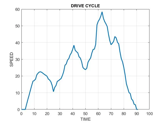
                                                                                                                                     FIG 1: Drive Cycle

                                     

                                                                                                       Fig 2.1: Displaying the total braking energy

Verifying with excel calculation: 

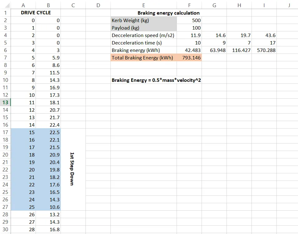                                                                   Fig 2.2 Braking Energy Excel Sheet Calculation

In both the calculations, we get the same total braking energy. So, our objective is proved successful.

Q.2.  Why electric motor can’t develop braking torque at a high speed similar to starting? How electric and mechanical brakes are coordinated? 

Answer:   

                                                                   Fig. 3

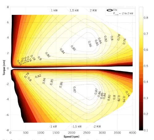Fig. 3 Represents the two quadrants of the motor operation where in the first quadrant both torque and speed are +ve (Forward motoring) and in the second quadrant the speed is +ve and the torque is –ve. (Braking)

At High speed, the torque will be less & operates at a constant power region hence it is difficult to bring the vehicle to rest or decelerate immediately. The peak acceleration torque is greater than the peak deceleration torque.  Hence Braking torque of the EV motor is not as high as the acceleration Torque.

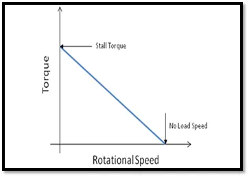                                                                                         Fig 4

DC motor Torque vs Speed Characteristic

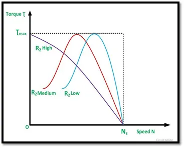                                                                                       Fig 5

Here for both in the case of AC or DC, there is no torque at maximum speed, gradually the torque decreases at high speed as the speed tends to be maximum. This situation does not occur at the beginning of acceleration because most of the torque is used to increase the kinetic energy of the load (and motor). But when the speed is already high and no extra load is applied it is not possible to increase the torque as well as to develop braking torque. The braking operation happens in the motion which is been distributed as per proportion in the Brake Energy and the regenerative braking.

The term braking comes from the term brake. We know that brake is a piece of equipment to reduce the speed of any moving or rotating equipment, like vehicles, locomotives. The process of applying brakes can be termed braking. Now coming to the term or question what is braking. First of all, we can classify the term braking into two parts

Mechanical braking is mostly used in scooters, motor vehicles, and motorcycles where small power is required. It is essential in manufacturing power transmission applications, material handling, etc. It delivers forces to the axle or a wheel to stop motion. It helps to reduce the speed of the system slowly by the mechanical process when compared to electrical braking. The working of a mechanical brake depends on the pedal. When the pedal is pressed, the brake shoes are pushed outwards and rotates against the drum which is connected to the wheels. Hence the machine or vehicle gets slow down and stopped. And when the pedal is released, it goes to a normal position due to the pullback action of spring shoes.

• Drum braking
• Disk braking
• Band braking
• Pawl and Ratchet braking

There are several types of mechanical brakes.

1) Band brakes: These are the simplest brake configuration, have a metal band lined with heat and wear-resistant friction material.

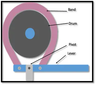                                                    Fig 6

2) Drum brakes: These are commonly used on automobile rear wheels, which work when shoes press against a spinning surface called a drum.

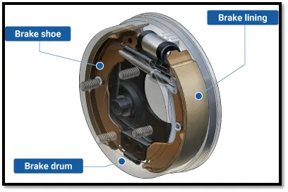                                            Fig 7

3) Disc brakes: These are constructed of brake pads, a caliper, and a rotor. During operation, the brake pads are squeezed against the rotor.

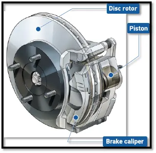                                                     Fig 8

Electrical Braking is used to reduce the speed of the machine depending on flux and torque. This type of braking is mainly used for functional braking to control the speed of the machine. It is easy to handle and comfortable. But it cannot be used for emergency braking and parking braking.

• Plugging type braking
• DC injection type braking
• Eddy current braking
• Dynamic resistor type braking
• Regenerative braking
• Sharing DC bus type braking

Electrical and mechanical braking systems can are coordinated by using a Brake strategy subsystem

1) Serial Braking Strategy

2) Parallel Braking Strategy

Implementation of serial braking strategy

Once the brake pedal is pressed and depending on the level of depression, brake torque is sent. Now, this brake torque passes into the brake control strategy block. Here, firstly it is checked if the battery state-of-charge is below 80% which is set as the maximum permissible level of charge. If that condition is satisfied, then the battery is recharged. The brake torque requested is compared to the maximum regenerative torque limit of the motor-generator. If the overall brake torque requested is less than or equal to the maximum regenerative torque, then the vehicle brakes purely on regenerative torque, and the battery is charged. The amount of charge ultimately put in depends also on the motor-generator operation efficiency and the battery charging efficiency. If the overall brake torque requested is greater than what the motor-generator can provide, then the friction brakes kick in. Now since the vehicle is front-driven, it is checked if the total brake torque requested from the front is less than or equal to the maximum regenerative torque capability of the motor-generator. If yes, then front braking is provided purely by regeneration and rear (non-driven axle) by friction. Once the total brake torque request increases further, then front friction brakes (driven axle) comes into play in combination with rear friction brakes and front regenerative braking, to satisfy the overall brake torque demand. This has been represented in a flow chart manner in fig.9

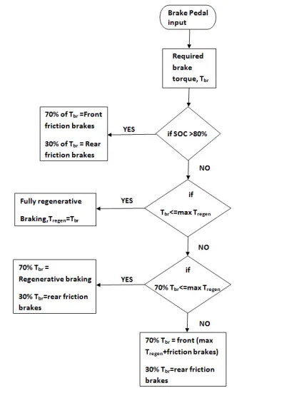                                                                                             Fig. 9

Implementation of parallel braking strategy

Once the brake pedal is applied and a desired overall brake torque request is sent from the driver block. This braking torque on passing through the brake control strategy gets divided between regeneration and friction braking at all times. The strategy is so modeled with the comfort and brake pedal feel in mind. As parallel regenerative braking is an add-on to conventional systems, it is devoid of any integrated control. So to make the transition and eco-performance of regenerative braking with friction smooth, it is assigned in such a way that, there is a clear division between the amount of brake torque that will be achieved from regeneration and friction braking. On application of brakes and in keeping with the design of the motor-generator, it is designed to operate the generator in a constant generator torque region. Motor-generator can provide a maximum of 322 Nm of generator torque at or under the base speed. The generator is scaled such that the base speed of the generator corresponds to a velocity of 124 [kmph], which is the maximum speed limit on most highways. Hence regeneration works, as long as the vehicle is braking from a speed of under 124 [kmph] and the requested brake torque on the front-driven wheels, after the front-rear brake split is greater than or equal to maximum generator torque. If that condition is satisfied, then regenerative and friction braking operates in tandem else it’s just the friction brakes at the driven and non-driven axle. This has been represented in a flow chart manner in fig.10

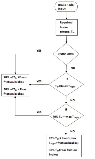                                                                                                      Fig. 10

Q.3. Make a MATLAB program that plots the contour of given motor speed, torque, and efficiency values.

Answer:   

MATLAB Code:

clear all
close all
clc
% Speed Array
omega = linspace(0, 300, 100);
% Torque Array
T = linspace(0, 2000, 100);
% Meshgrid
[X,Y] = meshgrid(T, omega);

% Loss Coefficients
cu = 0.17;               % Copper coefficient
fe = 0.006;              % Iron coefficient
win = 0.000015;          % Windage coefficient

% Losses
cu_loss = cu*(Y.^2);     % Copper Losses
fe_loss = fe*(X.^2);     % Iron Losses
win_loss = win*(X.^3);   % Windage Losses
cond_loss = 18;          % Conduction Losses

% Output Power
P_out = (X.*Y);
% Input Power
P_in = P_out + (cu_loss) + (fe_loss) + (win_loss) + (cond_loss);
% Efficiency
n = ((P_out)./(P_in));

% Efficiency values for contour
W = linspace(0.75, 0.95, 10);
% Contour Plot
contour(X,Y,n,W)
xlabel('Angular Speed, rad/s')
ylabel('Torque, Nm')
title('Speed, Torque and Efficiency characteristics of Motor')

Explanation:

In this MATLAB script, we create arrays for the speed and the torque of the motor using the ‘linspace’ command. For the speed, consider a range of values from 0 to 2000 radians per second whereas for the torque, consider a range of values from 0 to 300Nm. These arrays are then used to create 2D grid coordinates using the ‘meshgrid’ command. These coordinates will help in the creation of the contour plot. To find the efficiency of the motor, we need to consider the various losses that occur in the motor’s operation. These are:

• Copper losses
• Iron losses
• Windage losses
• Conduction losses

These various losses are dependent on the speed and the torque of the motor. They each also have a characteristic constant of proportionality which are all assumed for the following calculations and represented as 'K'. In each calculation, the speed and the torque are represented respectively as ω and T.

• Copper losses = KCu⋅ω2
• Iron losses =KFe⋅T2
• Windage losses =Kw⋅T3

The values of coefficients are taken as general values. Conduction losses are assumed to be 18 Joules.

Finally, we plot the contour with the 'contour' command. Besides, an array for the efficiency values we want to plot for is created called 'W' and is assigned for values ranging from an efficiency level of 0.75 to 0.95. This array is used in the creation of the contour. Axis labels and a title are also made for better readability.

Output:

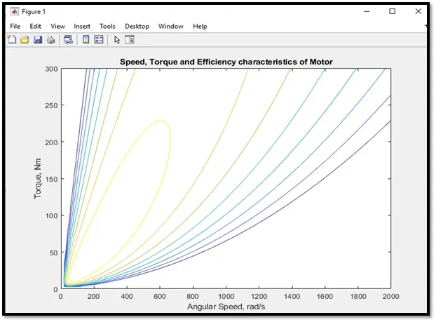                                              Fig 11

From this contour plot, we can see that the highest level of efficiency arises in the innermost contour plot and this efficiency decreases as the contours increase in size from the innermost contour.

Conclusions: All the problem statements are answered successfully with all the required calculations and plots.