Week-11 Challenge: Braking

Study 1 - For a defined driving cycle, calculate the energy required for braking.

Driving cycle is a series of data point representing the speed of a vehicle versus time. It has acceleration and deacceleration points means where velocity increases and decreases with respect to time. for deacceleration points braking is responsible. for these points we can calculate breaking energy as well.

Breaking energy is the kinetic energy which must be removed from moving object, to stop it. Generally breaking energy is given by the following formula –

`E_(br )`= `½*m*v^2`

We are going to use Indian urban duty cycle to calculate braking energy.so for we wrote a matlab script as following-

clear all
close all
clc
% read indian urban driving cycle
d = readmatrix('indian_driving_cycle.xlsx');

%Time(s)
t = d(:,1);

% Velocity(mph)
v = d(:,2);

%convert velocity mph to kmph
v = v*1.6*5/18;

% loop to calculate breaking energy
for j = 1:(length(d)-1)
  if v(j)>v(j+1)
    k(j)=0.5*50*(v(j)^2-v(j+1)^2)/(3.6*10^6);
  end
end


fprintf('total_breaking_power is %f KWh',sum(k));

%plot 
subplot(2,1,1)
plot(t,v,'linewidth',2)
xlabel('Time(s)')
ylabel('Velocity(mph)')
title('Duty cycle')
subplot(2,1,2)
plot(t(1:2690),k,'linewidth',2,'color','m')
xlabel('Time(s)')
ylabel('Breaking Energy(KWh)')

Result -

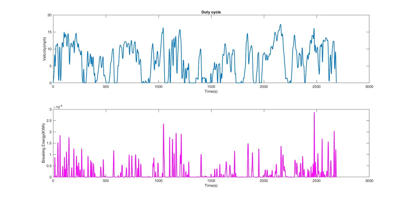
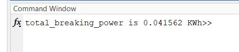
breaking energy for this cycle is -0.041562KWh.

Study 2 – Why electric motor can’t develop braking torque at high speed similar to starting? How electric and mechanical brakes are coordinated?

Regenerative breaking is or break energy recovery, is an important tool in the electrical vehicle arsenal, and when implemented correctly, can add more than 25% electric range to a vehicle.

The important consideration for regenerative breaking is how much electrical energy can be recovered to battery or how quickly the battery can accept charge. Well there is limitation of charging energy, after this limit battery temperature and voltage throws up their own limitation so it unlikely to get same energy which is consumed.

Electric motor generates torque based on rotation velocity, as the velocity increases from zero, there are three phases – sharp rise, flatlining and decrease with increasing speed, where the motor has reached its power limit. It is also true for negative velocity.

When break pedal is pressed, regenerative brake torque builds steadily and after certain time, at a particular speed, peak torque is reached due to recharging limit of battery and motor power limitation. As speed approaches to zero, the regenerative break drops all together and friction breaks come to play.

Coordination of mechanical and electric break –

Blending of electric and mechanical break is essential for smooth braking experience. At low deceleration levels, requested breaking can be achieved with electrical torque.at higher deceleration levels the blending workload increases and sharp changes in electrical torque can cause the friction some difficulty in keeping up.so for desire breaking proper coordination of mechanical and electrical break is very important.

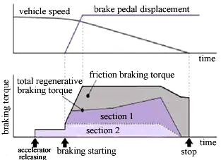
Electric and mechanical break can be connected in series or parallel connection. Most hybrid vehicles use an electrohydraulic system to achieve required breaking. Applied force on break pedal is read by pressure sensors which transmits a signal to break control unit. Control unit calculates desired friction to regen. Ratio. Since control parameter is changing, feedback system is also provided. According to friction to rgen. Ratio, control unit generates return signal and breaks performs their individual task.

Study 3 – Make a MATLAB program which plots contour of given motor speed, torque and efficiency values. Attach the code as a .m file attach a screenshot of all the plots

Matlab script –

close all
clear all
clc

% define torque, speed values
v = linspace(0,1000);
t = linspace(0,250);

%define constants
k_i = 0.008;                   % iron losses constant
k_c = 0.2;                     % copper losses constant
k_w = 0.00001;                 % windage losses constant
c_l = 20;                      % constant losses

% make meshgrid
[V,T] = meshgrid(v,t);

%calculate losses
l_c =  k_c*(T.^2);             % copper losses
l_i = k_i*V;                   % iron losses
l_w = k_w*(V.^3);              % windage losses
t_l = l_c + l_i +l_w + c_l;    % total losses

%Power ouput
p_out = T.*V;

%Power input
p_in = p_out + t_l;       

% calculating efficiency
n_c = p_out./p_in;

%efficiency values
n = linspace(.70,0.95,10);

%plot contour
%box off
%grid off
contour(V,T,n_c,n);
xlabel('Torque(N/m)')
ylabel('Speed(rad/s)')
% power
p=[8000,10000,15000];
hold on
contour(V,T,p_out,p);

Result -

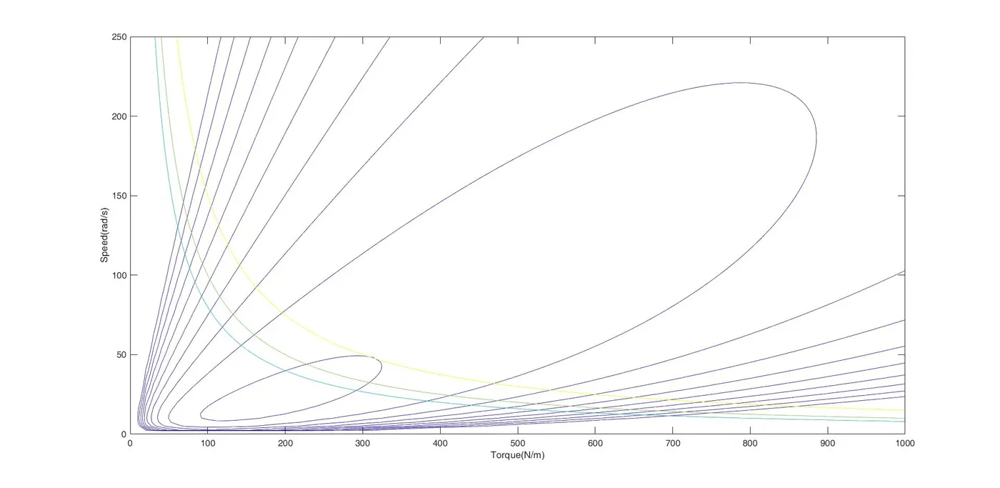
We got following contour plot. It has loops which represents same efficiency, like inner most loop representing 95% efficiency for different values of torque and speed which lies on this loop. there are three hyperbolic lines also which represents power values 8KW, 10KW, 15KW.

The following link contains matlab script files -

https://drive.google.com/file/d/1d9_qfxB8T8zac-JNFj-ybq3dtUcwgk7V/view?usp=sharing

https://drive.google.com/file/d/1wcJz_B6zAeLIwxjpC4sEZZegsssNPjWU/view?usp=sharing