Week-11 Challenge: Braking
DRIVE CYCLES:
A driving cycle is a series of data points representing the speed of a vehicle versus time. Driving cycles are produced by different countries and organizations to assess the performance of vehicles in various ways, as for example fuel consumption and polluting emissions.
In this challenge we can take UDDS drive cycle for the brake test.
The above image is only example of the UDDS drive cycle.
LINK FOR THE DRIVE CYCLE DATA:
https://drive.google.com/file/d/16-Nckl3aUGQ81ov_yVemkWNHHMIZ_7oe/view?usp=sharing
CALCULATION:
(J)
where,
m=mass of the vehicle(payload+kerb weight),
m=1000kg,
v=velocity(km/h).
In case of braking the high speed is reduced to low speed, so
(J)
where,
= final velocity(m/s),
= initial velocity(m/s),
By substituiting the values in the above formula, we can get a output in the form of joules.
To convert joules to Kwh we can divide the output by 360000.
The brake power required for the vehicle to stop from 57kmph to 0kmph is about 0.0348 kWh.
2.ELECTRIC MOTOR BRAKING:
The electric motor braking is done through the process called as Regenerative Braking.
In this process, when a brake is applied the power supply to the motor cut off and the friction brakes are actuated. From this the flow of the current is reversed using a Bidirectional Inverter and the energy is saved to the battery.
current flows through the electric motor, a related electrical charge causes an armature to rotate. These rotations within an internal magnetic field cause something called a back-EMF (electromotive force) which opposes the supply voltage. Imagine back-EMF to be the equivalent of a natural braking force, much like in IC engines.
From the above graph the spped and the torque of a elecrtic motor is plotted.
At zero speeds the torque is so high and it is called as constant torque region. In this region the torque produced is constant for a typical speed of a motor operates.
At rated speeds the torque cuve is gradually dropped and enters the constant power region and also called as critical speed point.
When applying the brakes at hifh speeds to zero speed the motor operates at the constant power region and the braking torque produced is very low. So the motor can't able to create max torque while braking.
BRAKE CONTROL STRATEGIES:
To stop the vehicle at shorter period of time W.R.T.speed and torque the regenerative and frictional brakes are used at both times.
This happened by senting signals to both hydraulic system and the power converter system(inverter).
There are two types of braking combos used in electric vehicles, they are
Series combo, both the brakes actuated one after another. This is based on comfort of the driver and the efficiency of the vehicle.
Parallel combo, both the brakes are actuated at the same time. This type saves lot of energy.
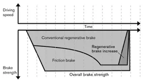
And there is an other technology used in braking of the electric vehicles, that is Electric Driven Intelligent Braking System(EDIB).
WORKING OF EIDB SYSTEM:
After stepping on the brake pedal, the system produces natural and adequate braking force that corresponds to the operation. The amount of energy regeneration also needs to be increased as much as possible.
EDIB controls the regenerative brake and friction brake to support both of these requirements. Further, it also controls the reactive force from the pedal in order to unify the feeling when stepping down on the pedal and the sense of deceleration.
3.MOTOR'S SPEED TORQUE AND EFFCIENCY:
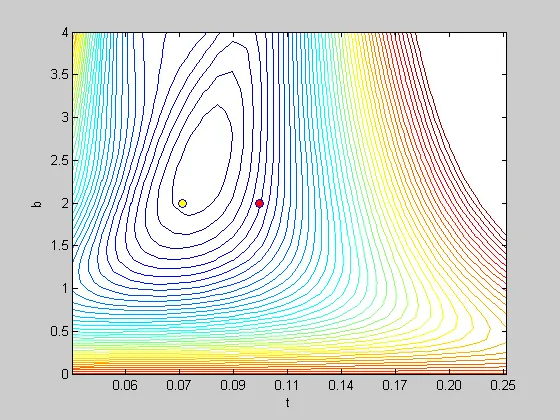
The efficiency of the simple DC motor is plotted in a contour style for the given range of speed and torque values respectively.
CONTOUR PLOT IN MATLAB:
A contour plot is a graphical technique for representing a 3-dimensional surface by plotting constant z slices, called contours, on a 2-dimensional format. This contour plot shows that the surface is symmetric and peaks in the center.
TYPES OF LOSSES:
Copper loss:
It is expressed as [(I^2)*R]
where, the current is proportional to the torque. So the equation is given as,
I^2 . R = K_c*T^2
where
K_c=copper loss constant,
T=torque(N-m),
I=current(A);
R=resistance(ohms).
Iron loss:
It is given by K_i*omega
where,
K_i=iron loss constant,
omega=speed(rad/s);
Wintage loss:
It is given by K_w*omega^3
where,
K_w=wintage loss constant.
Constant loss:
For every motor there are some constant losses takes place and it is denoted as(c).
MATLAB CODE:
clear all
close all
clc

%input arrays
speed = linspace(0,1000);
torque = linspace(0,250);

%input for motor loss constants
k_c = 0.2;%copper loss
k_i = 0.008;%iron loss
k_w = 0.0001;%wintage loss
constant = 20;

%creating a meshgrid
[X,Y] = meshgrid(speed,torque);
Output_power = (X.*Y);
cu_loss = (Y.^2)*k_c;
iron_loss = k_i*X;
wintage_loss = k_w*(X.^3);

Input_power = Output_power+cu_loss+iron_loss+wintage_loss+constant;

Efficiency = Output_power./Input_power;

%range of values
V = [0.70,0.75,0.80,0.85,0.89,0.91,0.93];

%plotting speed torque Efficiency
box off
grid off
contourf(speed,torque,Efficiency,V);
colorbar
xlabel("speed(rad/s)");
ylabel("torque(N-m)");
zlabel(Efficiency);
title("contour of motor speed torque Effciency");
OUTPUT FOR THE PROGRAM: