Simulating Combustion of Natural Gas

Aim:-

• Perform a combustion simulation on the combustor model.
• Plot the variation of the mass fraction of the different species in the simulation using line probes at different locations of the combustor.
• Also, plot contour plot for CO2, H2O, CH4, N2, O2, NOx emission, and Soot Formation.
• To reduce Nox and soot formation at the outlet check the effect of adding water to the fuel.
• Add the water content in fuel from 5% to 30% by mole and observe the effect of it on the results.
• Finally, plot the line graphs and contour charts to observe the change.

Objective:-

• Simplify the geometry model into a 2D geometry model to save cell counts and time required for simulation.
• Apply mesh on that 2D Combustor model.
• For the first observation Set up the simulation model to analyze the combustor model. (use methane-air-2 step as a mixture material than methane-air which allows to add water in the fuel and use one-step soot model to calculate the soot formation).
• Plot the contour plots of mass fraction of different species.
• Then, using line probes at the different locations of the combustor plot line plot of mass fraction of those species.
• For the second observation, to reduce NOx and soot formation at the outlet check the effect of adding water to the fuel.
• Observe the effect of it on the pollutant NOx and soot by adding water with a range from 5% to 30%.
• For comparison, plot the NOx and soot plot of each species with each simulated range of the added H2O content.

Workbench Setup

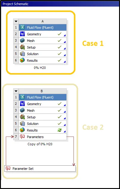
The workbench was set up to simulate 2 cases. The first case to simulate 100% fuel (natural gas) supply with air mixture. And for the second case, the water was added to check its effect on the reduction of pollutants and soot formations.

Geometry Cleanup

Geometry was cleaned up into the space claim of from fluent cell. The model was imported into the space claim design modeler. At the first look, geometry was a cylinder 3D model, therefore, it requires more number of mesh cells leads to large computational time and money. Hence, geometry is needed to be simplified.

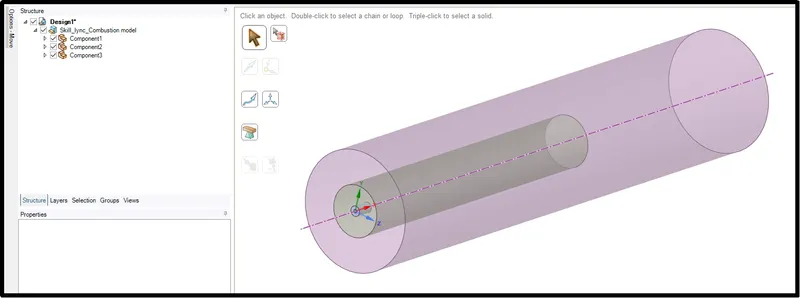
There are three axially symmetrical components present in the 3D geometrical model.

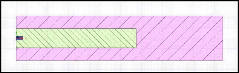
To extract the 2D plane surface, first, the model components were combined using the combine command.

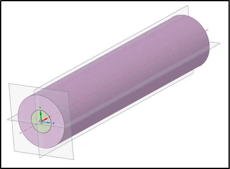
Then, the geometrical model was split in half using a midplane.

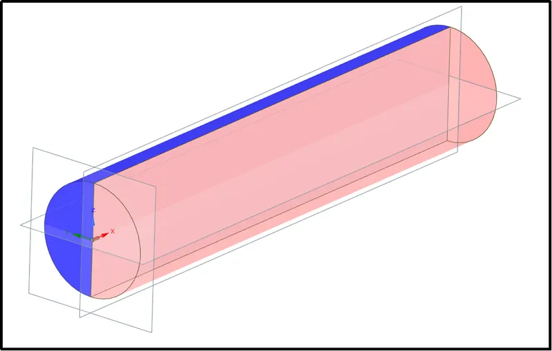
Afterward, it was again split in half as we require an axisymmetrical 2D cross-sectional area of the component.

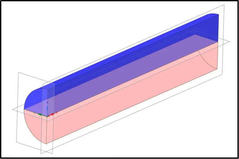
Lastly, the axisymmetrical cross-sectional surface was copied and pasted into the new space claim window.

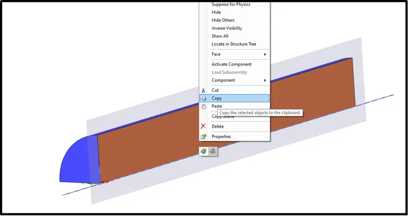
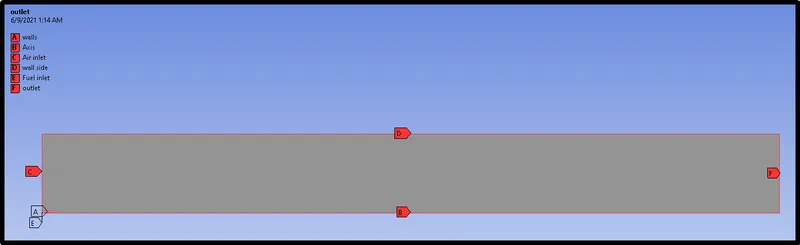
In Ansys fluent, in order to consider axisymmetric approximation one has to paste geometry on the X-Y plane, and the axis should be along the X-axis. After, geometrical cleanup using the above method we got the following 2D axisymmetrical cross-section for further support.

Boundary definition:-

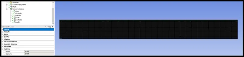
All edges were defined to apply boundary conditions in a fluent setup. at entry, there are two inlets larger edge is for air inlet and a small inlet for fuel. Additionally, one Axial edge was defined and one outlet was defined.

Computational mesh:-

Element size of 0.89 was used to mesh the model with even quad mesh.

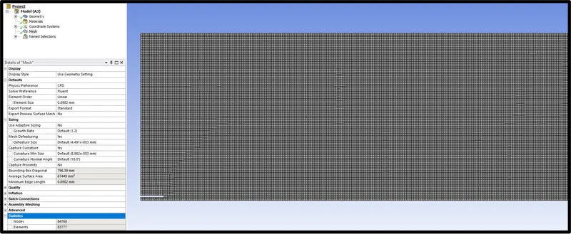
Total elements count was maintained below 512000 element which is 85777 number of cells.

Fluent Setup for Case1:-

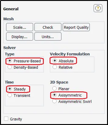
A pressure-based solver was used with absolute velocity formation considering the steady-state conditions.

This is the axisymmetrical model, hence, axisymmetry was turned on

Basics of combustion simulation

Equation solved for Mass, Momentum and Species Transport Equation(Source terms is computed using the combustion model)

`(del)/(del t) (rho Y_i) + Delta.(rho vecv Y_i) = - Delta. V_(ecv)j_i + R_i + S_i`

`(del)/(del t) (rho Y_i)` -> Time Derivative

`Delta.(rho v_(ecv) Y_i)` -> Convection

`Delta. Vecj_i` -> Diffusion (Motion due to concentration gradient)

`R_i + S_i` -> Sources (Reaction + User defined)

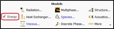
This simulation is related to the combustion process therefore we need to turn on the energy equation

Laminar and Turbulent diffusion

Diffusion is a combination of laminar and turbulent diffusion. Typically, for engineering applications (IC Engines, Gas turbines, Large Burners) Turbulent diffusion >> Laminar Diffusion. So, we use Fick's Law (Dilute approximation)

If the flow is purely laminar (for Example, laminar flames) then Fick’s law is not valid and we need to include the multicomponent diffusion properties.

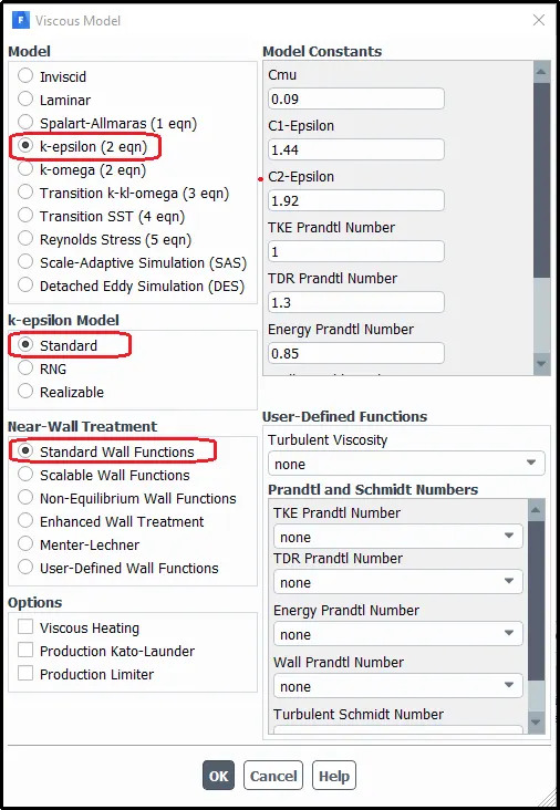
Combustion:-

Combustion is a high-temperature exothermic (heat releasing) redox (oxygen adding) chemical reaction between a fuel and an oxidant, usually atmosphere oxygen.

Possible types of combustion simulation that we can perform using Ansys fluid:-

Primarily there is two main classification

[A] Based on the mixing of air and fuel mixture

> Non-premixed combustion (Direct injection, Late injection)

Fuel is injected just before combustion starts. In essence, a diesel engine where fuel is directly injected inside the cylinder and starts to burn as it is mixed with the hot compressed air.

> Premixed combustion (Carburetor)

In this case, the air-fuel mixture is already mixed in the carburetor, in IC engines, before entering into the engine cylinder for combustion. This process gets more time to vaporize and properly mixed with the air which leads to a very uniform mixture.

> Partially Premixed

This category comes in between premixed and non-premixed.

[B] Based on Phase

> Fluid Phase (Volumetric reaction)

> Wall (surface reaction)

> Particles (surface reaction)

> Porous region ( Example: After treatment system)

Combustion source calculation:-

> Finite Rate Chemistry

• Accurate but slow

> Mixing based models

• The eddy Dissipation Model
• Fast but requires user experience.

> Finite Rate Eddy Dissipation Model

• Combination of both Finite Rate chemistry and Eddy Dissipation model
• Used to prevent instantaneous burning (mixed is burnt problem)

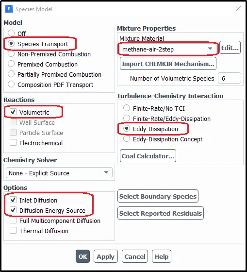
In the Species model species transport was selected with volumetric reaction and inlet diffusion and Diffusion energy source option was turned on. in mixture material 'methane-air-2step' mixture material was used which allows to add water in the fuel or air.

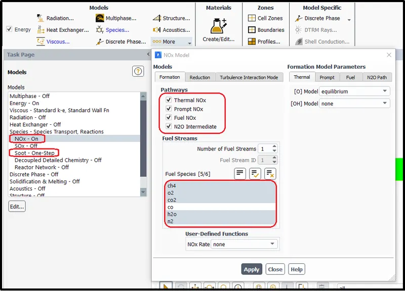
To find out other NOx pollutants and soot formation in simulation that model was turned on in more models option in fluent setup.

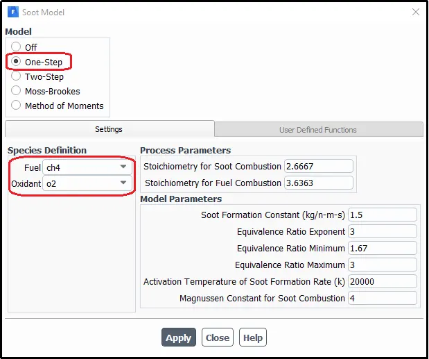
the one-step soot model was used for this simulation with the Fuel as CH4 and Oxidant as O2.

Boundary condition:-

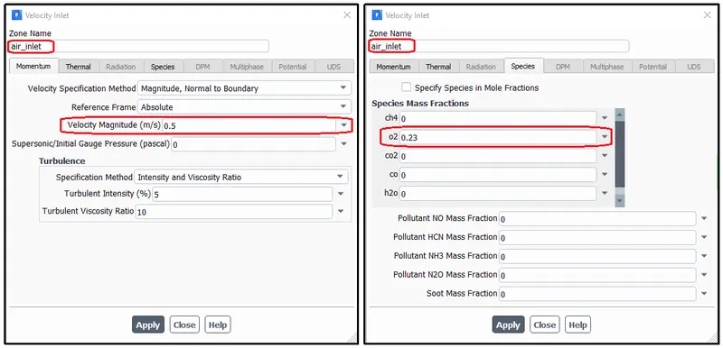
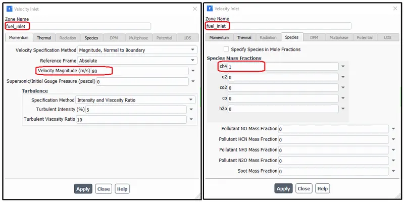
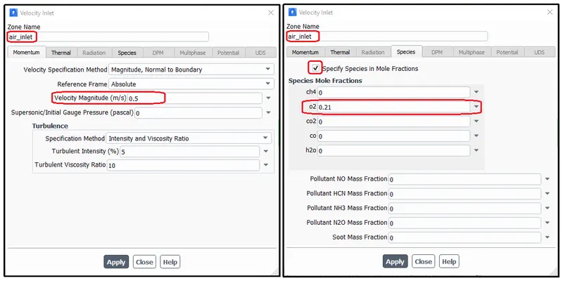
In boundary condition setting air, inlet velocity was set to 0.5m/s and fuel velocity set to be 80m/s. To observe combustion reaction one needs to specify the mass or mole fraction of the species involved in the reaction process.

At air inlet, the velocity inlet is given as 0.5 m/s with 0.23 mass fraction of o2

Air is consist of approx 21% oxygen and 79% nitrogen

So chemical formulation of the air-fuel mixture will be

CH4 + ar(O2 +3.76 N2) --> a CO2 + b H2O + c N2

Therefore,

a = 1

4 = 2b

2ar = 2a + b

ar = a + b/2 = 1 + 1 = 2

Then,

Air = 2 mole of O2 + 7.52 moles N2

After adding the moles of air

2 mole of O2 + 7.52 moles N2 = 9.52

Mole fraction

> Molar fraction of O2 = 2/9.52 = 0.21

> Molar fraction of N2 = 7.52/9.52 = 0.79

Mass Fraction from mole fraction

> Molar mass of O2 = 32 g/mole

> Molar mass of N2 = 28 g/mole

Mass fraction of species = Molar fraction of species x molar mass of species

Mass of O2 = 0.21 xx 32 = 6.72g

Mass of N2 = 0.79 xx 28 = 22.12g

After adding the moles of air

6.72g O2 + 22.12g N2 = 28.84g

Mass fraction of O2 = 6.72/28.84 = 0.233

Mass fraction of N2 = 22.12/28.84 = 0.767

Consider

Fuel = 1mole of CH4 in case 1

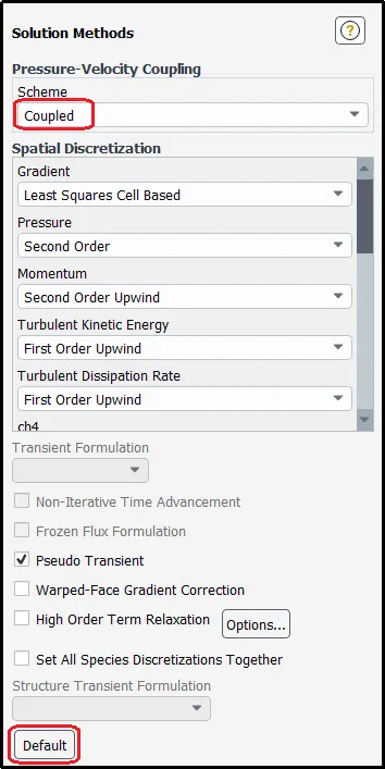
A fluent default solution method was used to run the setup.

Initialize the setup - Hybrid initialization

The hybrid Initialization method is an efficient method of initializing the solution based purely on the setup of the simulation with no extra information required. These methods produce a velocity field that conforms to complex domain geometries and a pressure field that conforms to complex domain geometries and a pressure field that smoothly connects high and low-pressure values.

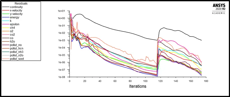
In this case, the solution is converging at the 174^th iteration

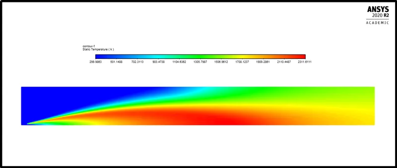
Static Temperature of combustor 2D plane:-

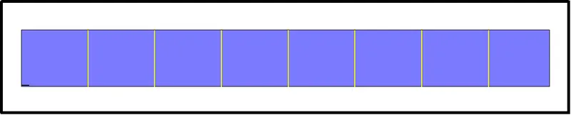
line probes

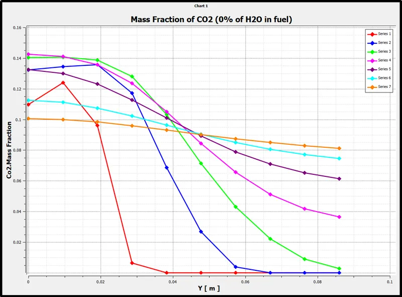
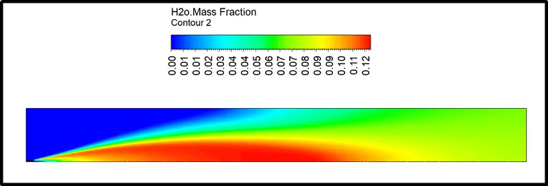
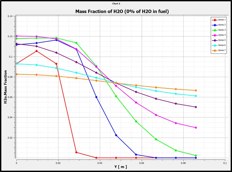
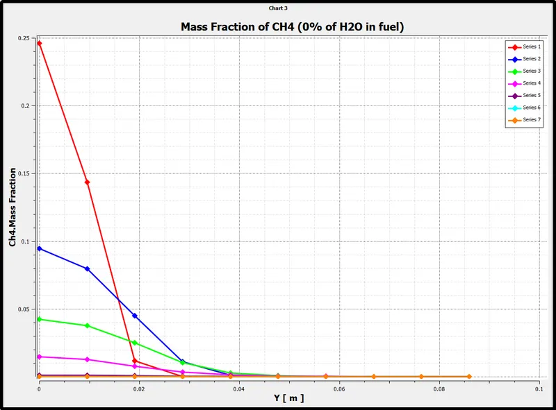
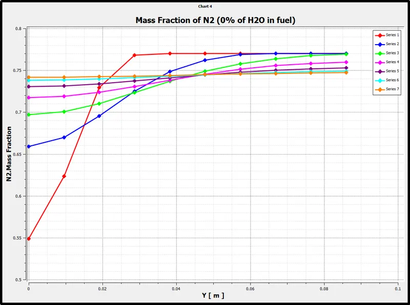
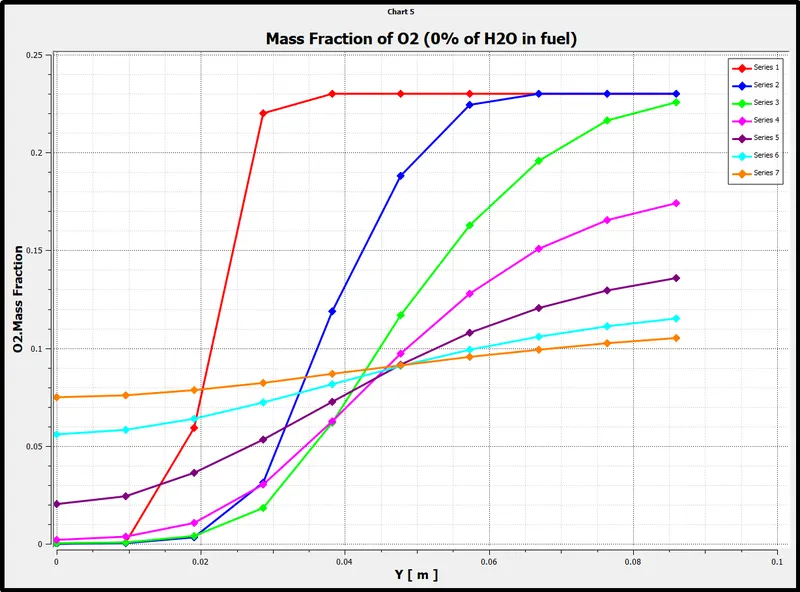
line probes were used at different locations of the combustor, to observe the variation of the mass fraction of the different species in the simulation. There are seven monitor line probe placed with the distance of 1m from each other as exhibited in below figure.

Variation of mass fraction of all the species:-

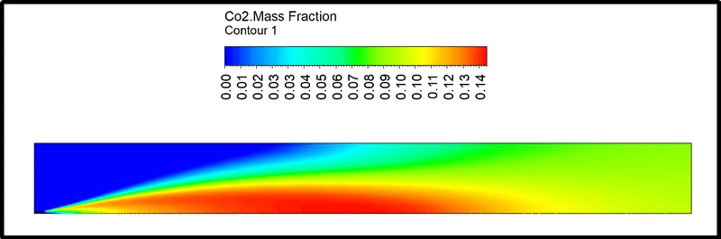
Contour plot of mass fraction of CO2

Mass fraction variation of CO2 on each monitor line

Contour plot of mass fraction of H2O

Mass fraction variation of H2O on each monitor line

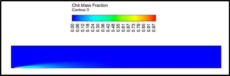
Contour plot of mass fraction of CH4

Mass fraction variation of CH4 on each monitor line

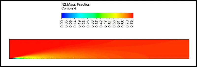
Contour plot of mass fraction of N2

Mass fraction variation of N2 on each monitor line

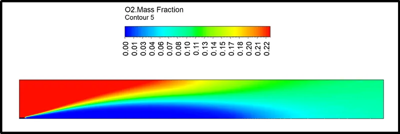
Contour plot of mass fraction of O2

Mass fraction variation of O2 on each monitor line

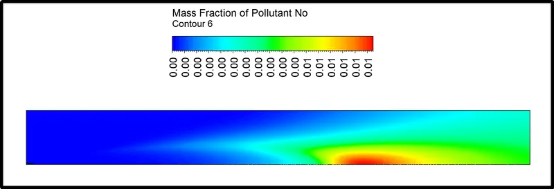
Contour plot of mass fraction of NOx

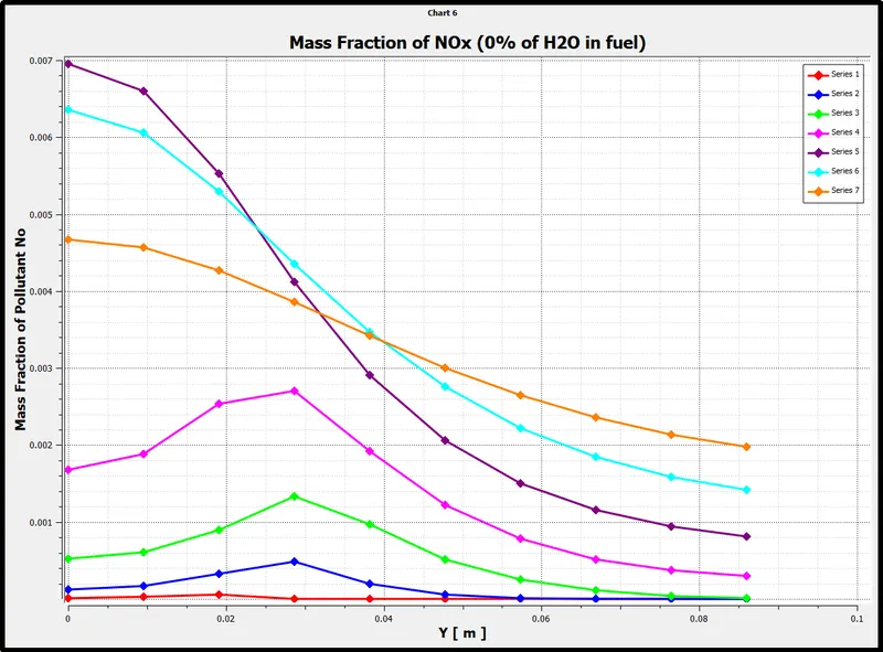
Mass fraction variation of NOx on each monitor line

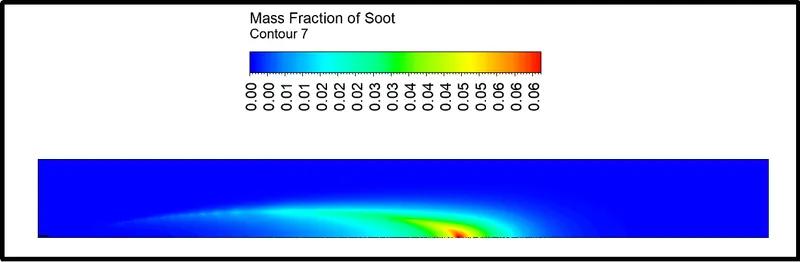
Contour plot of mass fraction of Soot

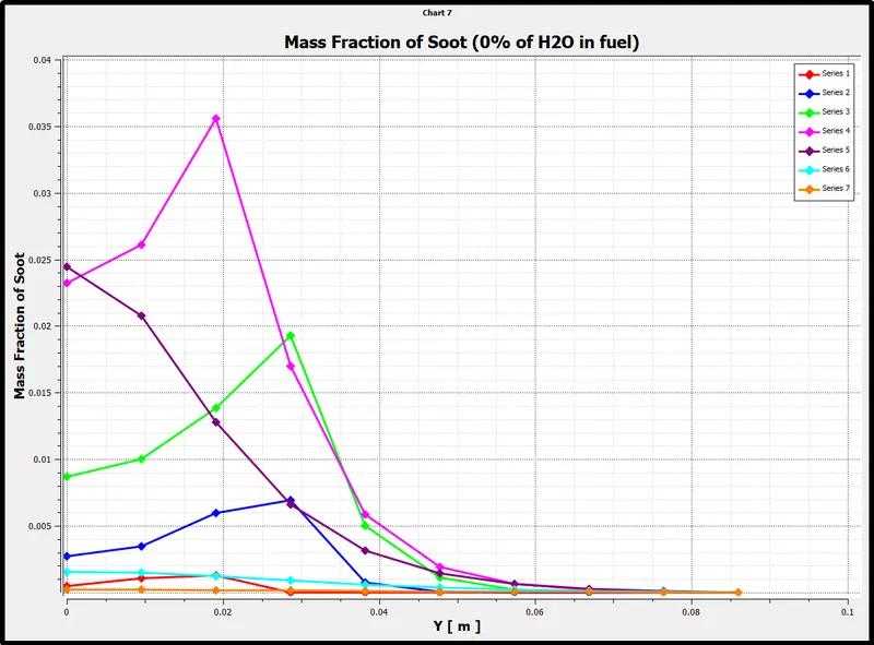
Mass fraction variation of Soot on each monitor line

Case 2

From the first case, we observe the NOx and Soot are getting formed at the outlet of the combustor. Such formation has harmful effects on the environment and humans. The stringent government norms also demand the least formation on NOx and Soot and to satisfy those requirements, to reduce NOx and soot formation, the effect of adding water in fuel should be observed in case 2

for the case 2 study, all fluent setting kept the same as the previous simulation except the fuel inlet setting here parametric setup was used to add water pecentace wise in between 5% to 30% range

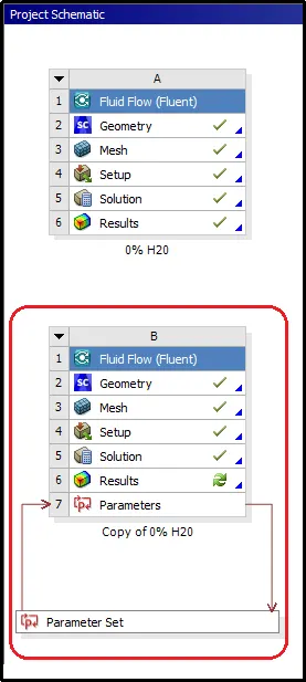
Fluent setup Case 2

In this case, the boundary condition was kept the same as before just this time the Species fraction was specified in the mole fraction.

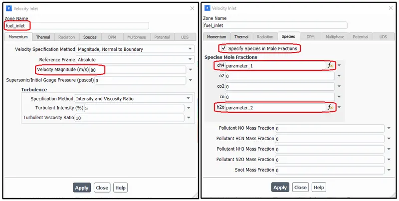
In a bid to reduce the soot and NOx pollutant formation, various simulations were performed by adding water by 5%, 10%, 15%, 20%, 25%, and 30% with each simulation. To save time parametric setup was used to simulate and compare each result.

Parameter_1 = Molar fraction of CH4

Parameter_2 = Molar fraction of H2O

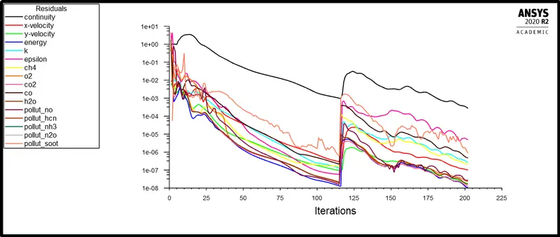
The simulation was performed using the default solution method using hybrid initialization and it ran up to 206 iterations.

Results of case2:-

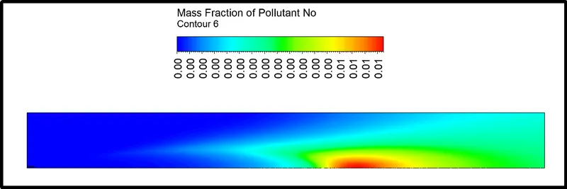
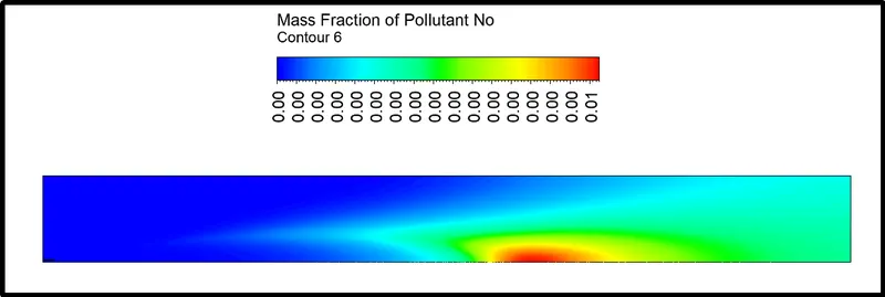
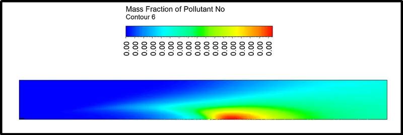
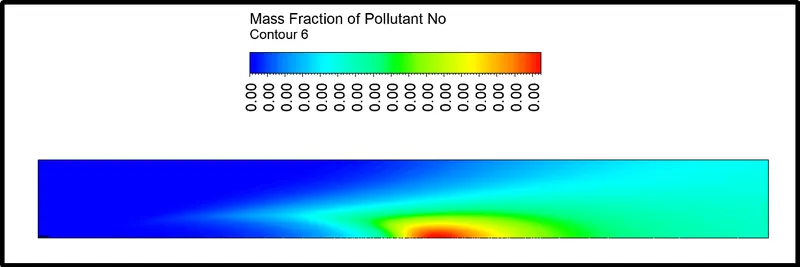
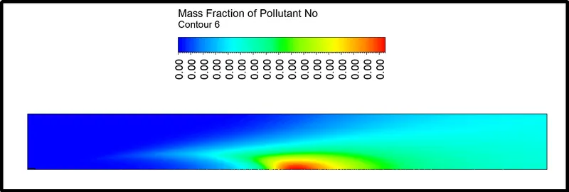
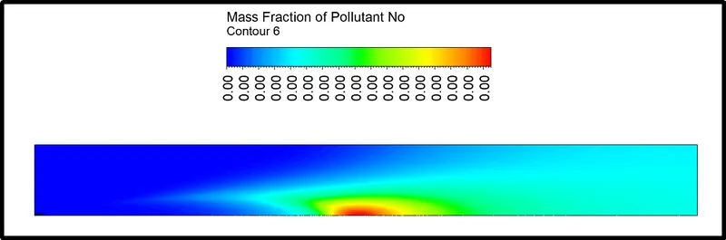
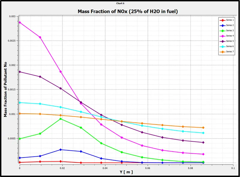
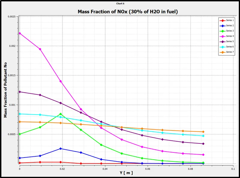
Effect of added water with 0%, 5%, 10%, 15%, 20%, 25%, and 30% in the fuel on the mass fraction of NOx with respective order.

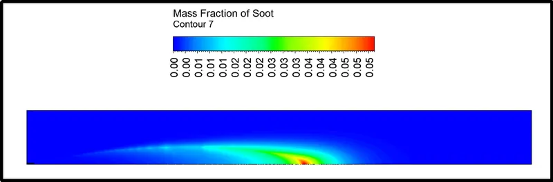
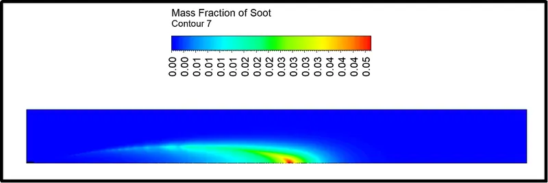
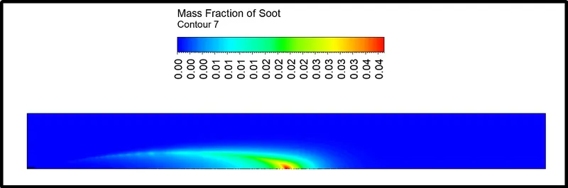
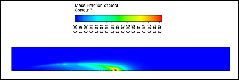
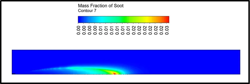
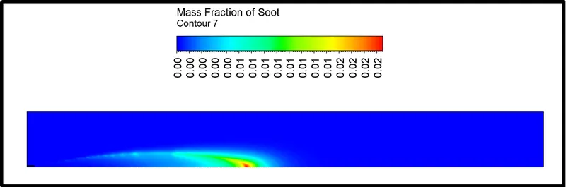
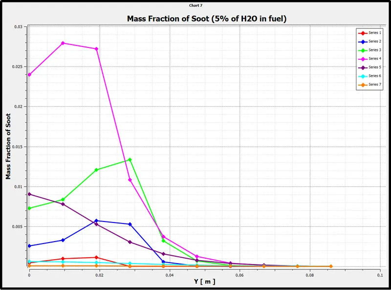
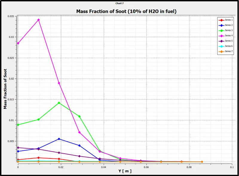
Effect of added water with 0%, 5%, 10%, 15%, 20%, 25%, and 30% in the fuel on the mass fraction of Soot with respective order.

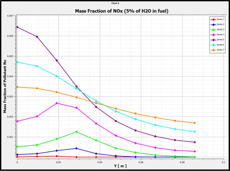
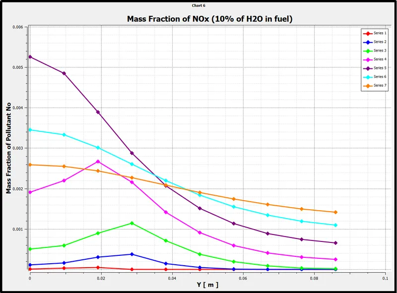
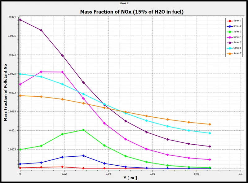
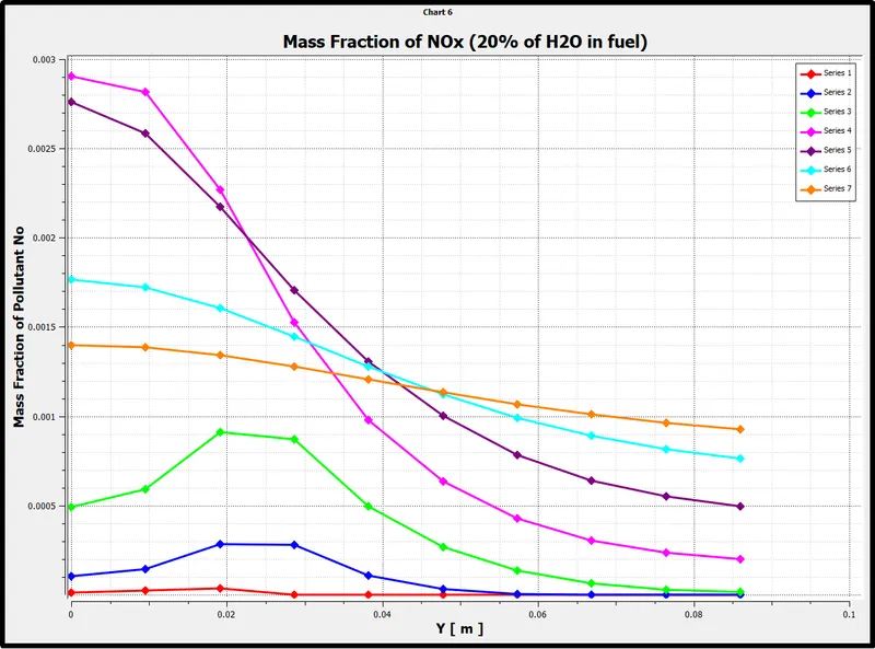
Comparison charts to observe the effect of added water from 5% to 30% on variation in mass fraction of NOx at each monitor probe in the combustor

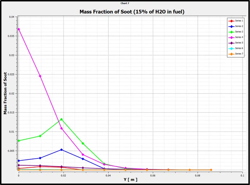
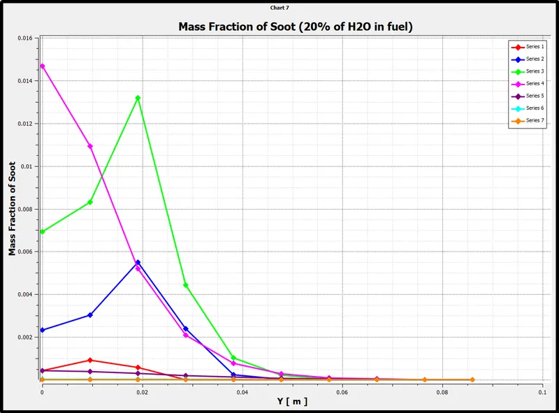
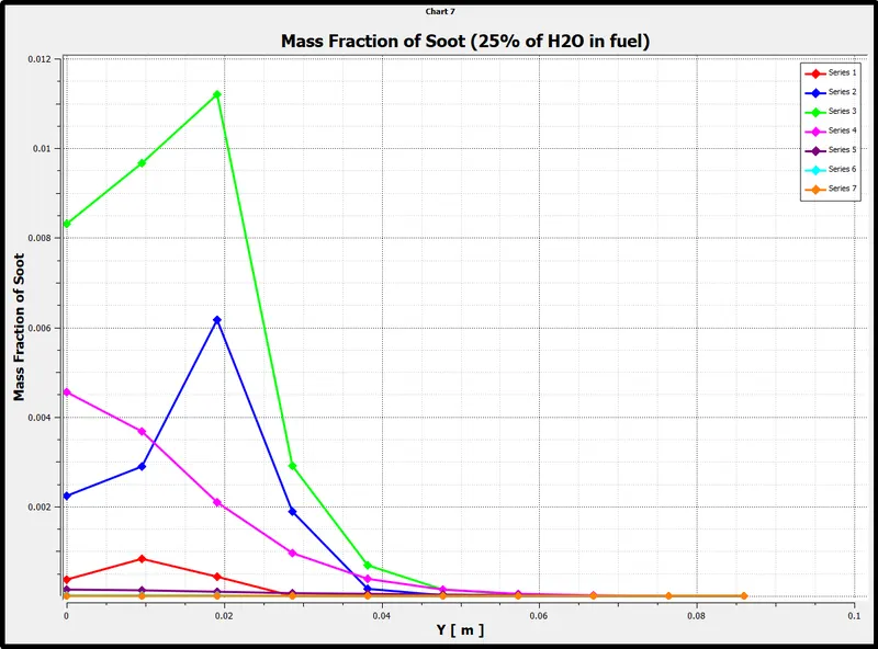
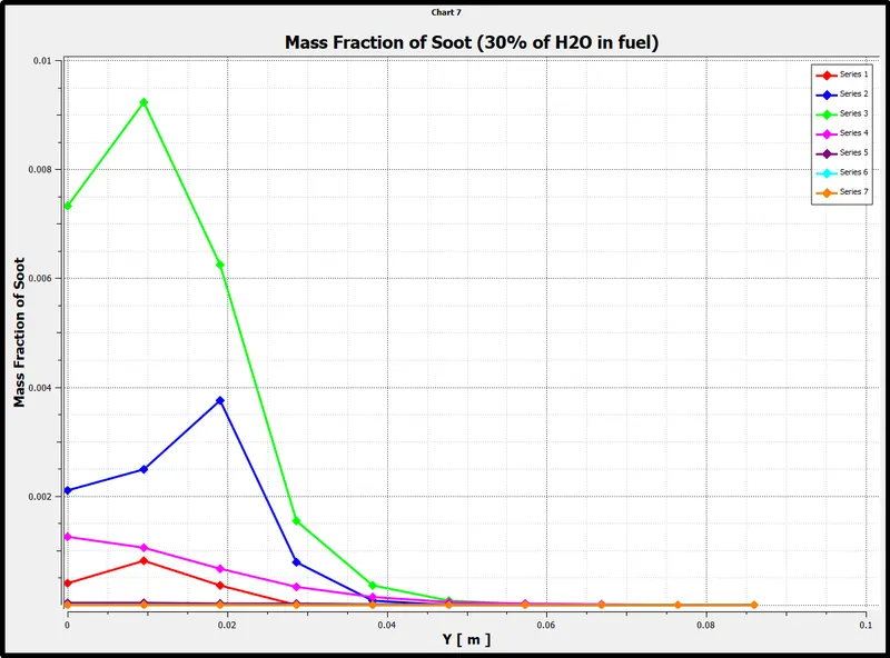
Comparison charts to observe the effect of added water from 5% to 30% on variation in mass fraction of soot at each monitor probe in the combustor

Observation Table:-

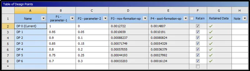
After observation of all the simulated results, all contour plots of Nox and soot, monitor line probe data line graph and above table one this is very clear to anyone that is, as the amount of water percentage increasing in the fuel the formation of NOx and Soot is reducing. In the above observation table, we can notice in the D and E column the NOx and Soot formation is reducing as the water content in natural gas is increasing.

Conclusion:-

• Geometry simplification and defeaturing are vital to reduce mesh cell count and reduce simulation time. as in this project, the 2D model of the combustor is enough to get desire results by using the axisymmetrical setting available in fluent.
• Defining proper combustion type in fluent setup is an important factor. An improperly defined combustion settings type can lead to wrong results.
• To reduce more time and manpower in simulation, the use of a parametric setting is a better idea in this type of project where all remaining results can be calculated with a single click. It also built a nice observation table by which users can easily compare all the result data.
• The main conclusion of this project is to find out the effect of water addition in fuel on the formation of NOx and Soot. So far, it is proven by our final observation charts, figures, and tables that the addition of water percentage in fuel leads to a reduction in the formation of NOx and soot.

References:-

[1] Modeling soot production and thermal radiation for turbulent diffusion flames - https://www.sciencedirect.com/science/article/pii/S1876610217337724

[2] An overview of systems supplying water into the combustion chamber of diesel engines to decrease the number of nitrogen oxides in the exhaust gas - https://link.springer.com/article/10.1007/s00773-015-0303-8