Week 10 - Simulating Combustion of Natural Gas.

Week 10 - Simulating Combustion of Natural Gas.

In this challenge,

• Part I - We perform a combustion simulation on the combustor model and plot the variation of the mass fraction of the different species in the simulation using line probes at different locations of the combustor. We will plot for CO2, H2O, CH4, N2, O2, NOx emissions & Soot formation.
• Part II -In this part, We add the water content in the fuel from 5% to 30% by mole and observe the effect of it on the results. We provide line plots and contours to prove our claim.We use the parametric study approach for this part.

Introduction:-

Before moving on to our main challenge, let's first go over some chemical kinetics basics and the fundamentals of combustion simulation in Ansys Fluent.

Chemical Kinetics:-

Every time we watch a reaction, it appears as though it happened in a single step, but this is not how reactions actually happen. Assume that fuel and air are combining. A specific operating temperature and pressure are maintained during the whole reaction. When fuel and air mix in these circumstances, it may result in various intermediate reactions. For instance, fuel may break down and join with oxygen in the air or other intermediate species. The elementary reaction is defined as the reaction between these intermediate species.
Such reactions frequently occur, and the collection of all such events and their intermediate species is referred to as the reaction mechanism.

Chemical kinetics is the study of the overall reaction mechanism under a variety of operating conditions.

In order to anticipate the ultimate products, whenever we utilise a chemical kinetics solver, we try to simulate the whole set of elementary reactions, the intermediate species, and the many trajectories the system can follow.
This means that the final products will entirely depend on the operating conditions and how long the combustion really lasts in practise. This reaction pathway is a function of time as well. This process will provide you with an accurate representation of the thermodynamic parameters following the combustion process if your reaction mechanisms and pathways have been computed appropriately.

In reality, the computer solver imports the complete reaction mechanism, including the data for the reactants and products. Experimental reactions can be used to determine these. The computer is loaded with all of this data. so that we can determine the thermodynamic parameters after combustion and that it can mimic the entire process (for emissions). But, in our scenario, the fluent solver already has the data.

• The chemical kinetics solver is important because the reaction pathways determine

1. Combustion start (ignition delay).
2. Heat release rate (Rate of work done).
3. Emmisions (How and how much pollutants are produced ).

Basics of combustion simulation :

Possible types of combustion (done using Ansys fluent) :

1)Based on mixing :

• Non - premixed (example - Direct injection , late injection)
• Pre - mixed (example - Carburetor,burner)
• Partially pre - mixed( In between premixed and non - premixed )

2) Based upon phase (where the combustion is taking place) :

• Fluid phase - If combustion taking place in fluid phase comes under this model and called it as volumetric reactions.For gas-phase reactions, the reaction rate is defined on a volumetric basis and the rate of creation and destruction of chemical species becomes a source term in the species conservation equations
• Wall surface -If combustion taking place on wall those type of reactions are called surface reactions. For surface reactions, the rate of adsorption and desorption is governed by both chemical kinetics and diffusion to and from the surface. Wall surface reactions thus create sources and sinks of chemical species in the gas phase, as well as on the reacting surface.
• Particle surface - Lagrangian particles on which reaction taking place is called particle surface reaction .Example - coal combustion .
• Porous region - Where reaction taking place in a porous region .Example - After treatment systems ,where we have a porous region where there is lot of pressure drop but also on top of it there is also reaction taking place.
• ANSYS FLUENT can model the mixing and transport of chemical species by solving conservation equations describing convection, diffusion, and reaction sources for each component species. Multiple simultaneous chemical reactions can be modeled, with reactions occurring in the bulk phase (volumetric reactions) and/or on wall or particle surfaces, and in the porous region. Species transport modeling capabilities, both with and without reactions.

Theory :

• In CFD in general we solve equations for mass , momentum and energy and in addition if there is turbulence we have equations for turbulence parameter(k,epsilon,omega).
• In addition to this if we have combustion going on we have reactants and products , together we call them as species .We need to solve an another equation called species transport equation for each species.
• When you choose to solve conservation equations for chemical species, ANSYS FLUENT predicts the local mass fraction of each species, , through the solution of a convection-diffusion equation for the th species. This conservation equation takes the following general form:

• where is the net rate of production of species by chemical reaction,

The reaction rates that appear as source terms in Equation (combustion source calculation ) are computed in ANSYS FLUENT, for turbulent flows, by one of the models:

1. Laminar finite-rate model: The effect of turbulent fluctuations are ignored, and reaction rates are determined by Arrhenius kinetic expressions.Here using chemical kinetics we basically calculate rate of production of each species ,we solve ODE for each species which is a costly process.Accurate but slow.
2. Eddy-dissipation model: Reaction rates are assumed to be controlled by the turbulence, so expensive Arrhenius chemical kinetic calculations can be avoided. The model is computationally cheap, but, for realistic results, only one or two step heat-release mechanisms should be used.Here the idea is , it is based upon turbulence quantities, it calculate mixing time scale based on turbulence quantities k and epsilon and combustion happens based upon the time scale. It does not need any type of ignition source ,ignition happens automatically based upon mixing time scale .It leads to ,mixing is burnt problem .It predicts results even where there is no combustion happens in reality. When you want to calculate ignition delay it shows wrong results as here there will be no delay in ignition , As mixture mixes it burns instantly.So even they are very fast it requires user experience .
3. Finite rate / eddy dissipation model : It is combination of both finite rate chemistry and eddy-dissipation model. Used to prevent instantaneous burning (mixed is burnt problem ) .Here we solve both and models and based upon flow condition which ever rate is going to have low reaction rate , the solver is going to pick that . IN certain areas where ignition is going to take place and ignition delay is important then model would ideally choose finite rate chemistry its much more suited for that and it may predicits low reaction rate and in things where turbulence play a much more major role , your reaction rate predicted by the eddy dissipation model is smaller and it picks that and let you know how reactants are getting converted to products .
4. Eddy-dissipation-concept (EDC) model: Detailed Arrhenius chemical kinetics can be incorporated in turbulent flames. Note that detailed chemical kinetic calculations are computationally expensive.

• And is the rate of creation by addition from the dispersed phase plus any user-defined sources. An equation of this form will be solved for species where is the total number of fluid phase
• chemical species present in the system. Since the mass fraction of the species must sum to unity, the th mass fraction is determined as one minus the sum of the solved mass fractions. To minimize numerical error, the th species should be selected as that species with the overall largest mass fraction, such as N when the oxidizer is air.
• In Equation J_i is the diffusion flux of species i , which arises due to gradients of concentration and temperature.
• Diffusion is a combination of laminar and turbulent diffusion.
• By default, ANSYS FLUENT uses the dilute approximation (also called Fick's law) to model mass diffusion due to concentration gradients.Here in dilute approximation we are looking at diffusion coefficient for each and every species how that species diffuses into entire mixture.
• For certain laminar flows, the dilute approximation may not be acceptable, and full multicomponent diffusion is required(Here we see diffusion coefficient of how each species react wih other species). In such cases, the Maxwell-Stefan equations can be solved.
• To explain shortly what happens is in each and every cell first the combustion model(finite ratechemistry/eddy dissipation model )is solved then based on that output (mole fractions etc.) obtained the species transport is solved..!

Simulation part :

Part I -

Here we perform a combustion simulation on the combustor model and plot the variation of the mass fraction of the different species in the simulation using line probes at different locations of the combustor. We will plot for CO2, H2O, CH4, N2, O2, NOx emissions & Soot formation.

Solution procedure :

• We wil simulate with the steady state.We will not simulate the 3D case because of the limitation af academic license.So, we are going to simulate 2D part . For solving we follow the below procedure :

1)Geometry setup

2)Meshing

3) Problem setup

4)Solving

5)Post processing

1) Geometry setup :

• In fluent module we have to open spaceClaim and then import the 3D geometry.The below image is the 3D view of gear box.

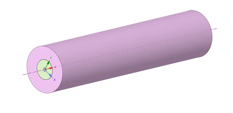
• If you take the entire geometry and simulate then , this is going to be much more expensive to simulate as we are going to have large number of cells.So we will perform 2D axisymmetric simulation .
• Now we have to split this body into half to extract the 2D geometry right in the middle plane.
• First create planes by selecting plane in design and click on origin ,which creates 2 planes X,Y and Z planes.
• We use the split body command in spaceclaim which is under design to split the geometry it into two parts by selecting the geometry and plane and delete the other part.
• Now we can see the interior sectional view.Now if you select the top part of the remaining geometry you can see the yellow top face part,which is what we want .Inorder to extract that area we need to select that face and copy and open new design and then paste it and save it.
• Now reset the setup and import the 2D saved geometry and open the meshing module.
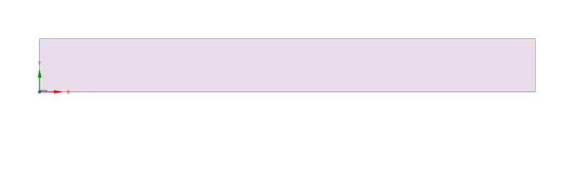
• The below image is the final 2D geometry that we simulate.

• Then we have to combine all the three parts using combine in design, then we get a single geometry .The below image is the final 2D geometry that we simulate.

• 2) Meshing :
• For meshing we open Meshing,where we mesh our model so that we can use it to solve our model.
• In general it is always good to name the surfaces before meshing. So let us do that.
• We have to give the name for air inlet , fuel inlet , walls , outlet , axis.
• We first select the axis (which is the X-axis line , to perform axisymmetric simulation the axis should be along X-axis ).using the edge selection so that we can provide name for our entity selection.
• steps : select the axis by using edge selection -> then press N -> name the selection as axis.
• In the similar way we name the air inlet , fuel inlet , walls , outlet.
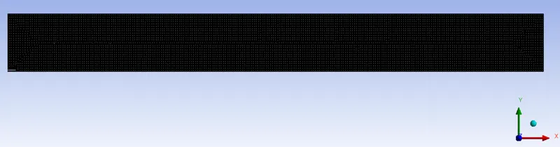
• Then next thing to do is to mesh.We click the mesh option in the side then give element size as 10 mm and also select capture proximity to on and generate mesh.
• The below image is the final view of mesh .

3) Problem Setup :

• To set up our problem we open Fluent and setup inital conditions , boundary conditions material etc.,
• We first start with checking the mesh quality using perform mesh check under domain.If no error is seen in console window then we can proceed further.
• Then we move move to setting up physics where we select the solver,viscous model etc.
• We use a steady state pressure based solver to solve our model.

Physics :

General :

Solver type : pressure based

2D space : Axisymmetric

time : steady state

velocity formulation : absolute

Energy : Enable

models :

viscous model : K-epsilon standard model with standard wall functions.

Species model :

model : species transport

Reactions : select volumetric

options : select diffusion energy source

In mixture properties ,

mixture material : methane- air. & methane-air-2step (respectively)

For, turbulence chemistry interaction : select eddy - dissipation

• We also select one-step soot model to calculate the soot formation and also select NOx model and enable thermal NOx in NOx model to calculate the NOx formation.

Zones :

Cell zone : In cell zones you will see fluid volume,it is of type fluid .

Boundary conditions :We will basically give our boundary conditions here such as inlet and outlet conditions.

we give,

air inlet :

momentum : velocity magnitude = 0.5 m/sec

thermal : temperature = 300 k

species : under species mass fractions give values ,for O2 = 0.23 and for remaining all species give zero (0) .

fuel inlet :

momentum : velocity magnitude = 80 m/sec

thermal : temperature = 300 k

species : under species mass fractions give values ,for CH4 = 1 and for remaining all species give zero (0) .

Outlet :

pressure outlet : gauge pressure = 0 pa

• For wall keep it as wall and for axis keep it as axis .
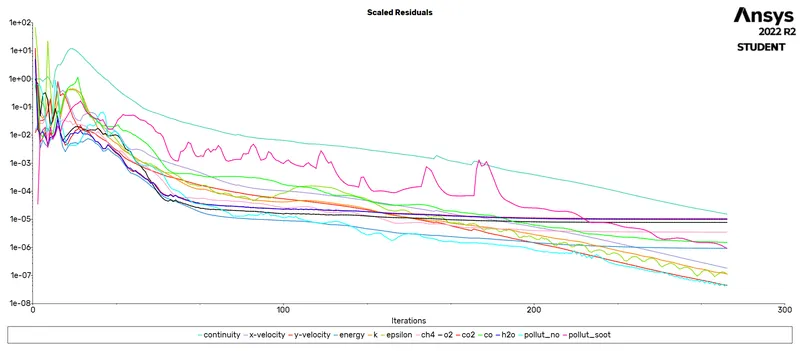
• In real life if you have burners like this ,the air and fuel only burn if you have an ignition source but in our case since we are using eddy dissipation model the fuel burning rate is not governed by the presence of energy source , it is governed by the presence of turbulence .If our k and epsilon are high enough its going to give a reasonable turbulence mixing time scale , based on which ansys fluent automatically calculates a time for combustion.
• Now we are almost ready to run the simulation ,but as the solution is being solved we want to moniter flow quantities while the solution is being generated.
• Here we want to moniter the temperature and emmisions( NOx and soot ) at the outlet .
• NOx - Nitrogen Oxides are a family of poisonous, highly reactive gases which causes pollution. These gases form when fuel is burned at high temperatures .
• Soot - A deep black powdery or flaky substance consisting largely of amorphous carbon, produced by the incomplete burning of organic matter which causes pollution .
• steps to create report for the temperature and emmisions ,

steps : solution -> under definitions -> select new -> select the surface report ->area weighted average-> and select the filed variable as temepreature and at surfaces we select outlet-> check report file and report plot ->then okay.

• In the similar way we also create report for NOx and soot formation at the outlet.
• we also want to create temperature contour and mass fraction contour for CO2, H2O, CH4, N2, O2 , NOx and soot . But before that we have to initialize the domain.We use the Hybrid initialization , this provides a very good initial condition .
• Then we create a temperature contour on the domain.

For contour -> go to solutions tab -> graphics -> contour -> in contour of : select temperature under that select static temperature -> select all the surfaces and press save /display.

• Then you can see the initial values for temperature which is obtained by initialization which is not the final one.
• In the similar way we also create contour for mass fraction of CO2, H2O, CH4, N2, O2 , NOx and soot.
• we also want to create amination so that as the solution is changing as the function of time we can see the physics behind it.
• Then we create animation so that we can see how the temperature is varying when problem is being solved.

For that,

steps : Activities -> solution animation -> select temperature contour ,which we have created -> preview -> set the required view and use active -> and name it as temperature animation.

• In solution method we use Coupled .

4) Solving :

• Give iterations such that our solution is converged.
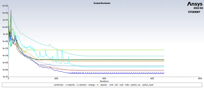
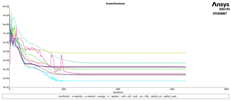
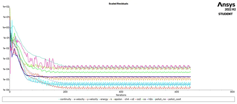
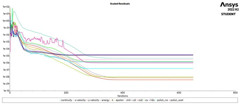
• Run the simulation until the steady state is reached.Lets run for 650 iterations , we can find the solution is converged.
• Then let us post process the results.

5) Post processing:-

1. For case setup with methane-air as fuel.

Plots and Contours of Mass Fraction related to that:-

1. Residuals plots

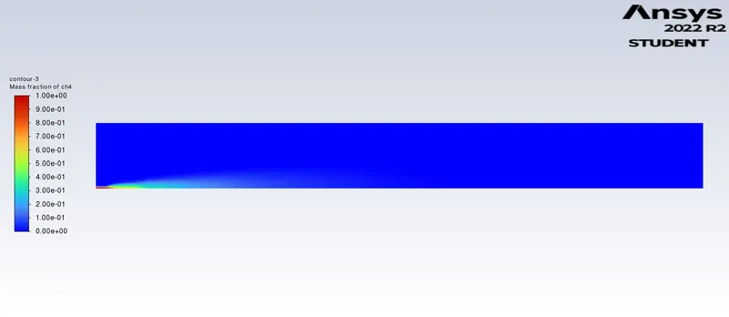
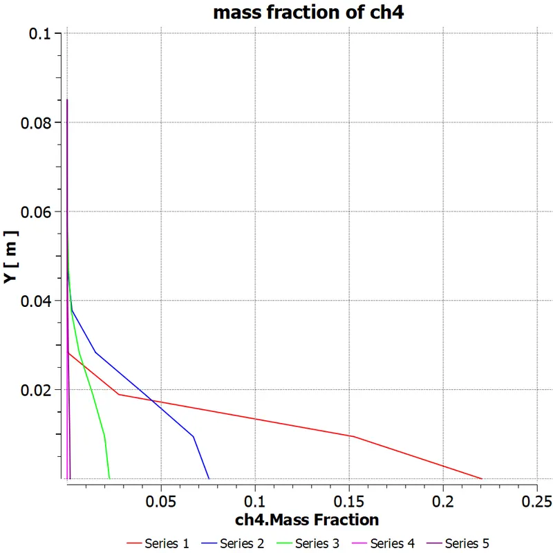
2. Mass fraction of CH4

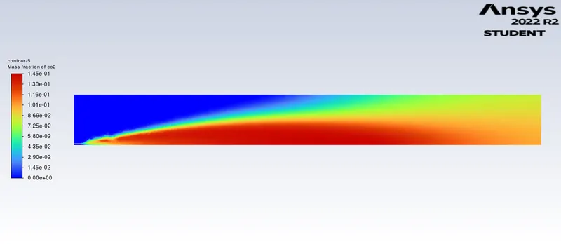
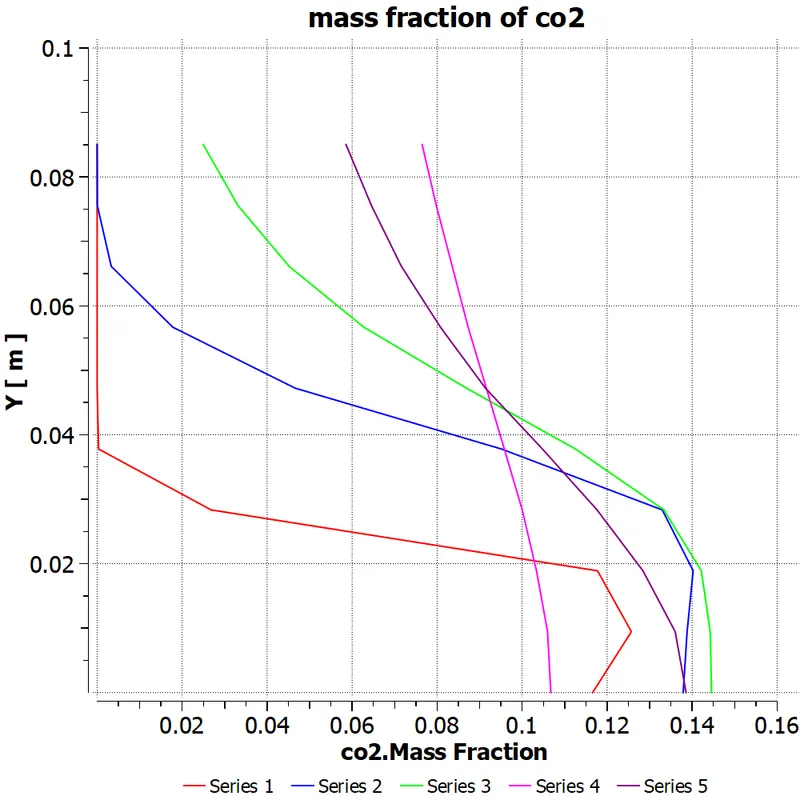
3.Mass fraction Of CO2

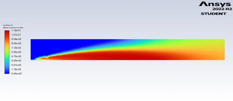
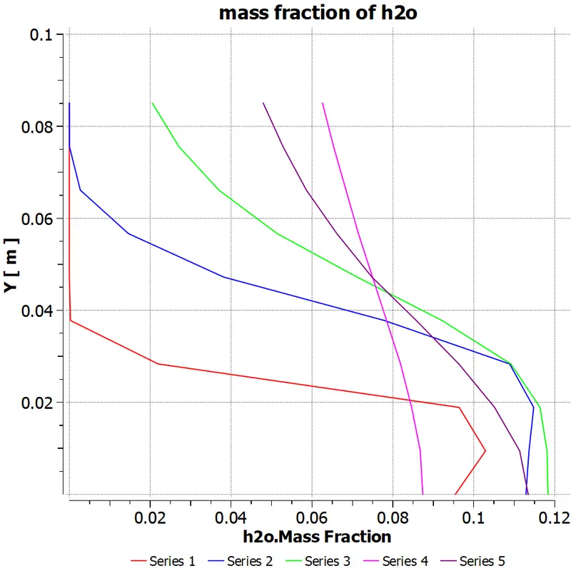
4. Mass fraction of H2O

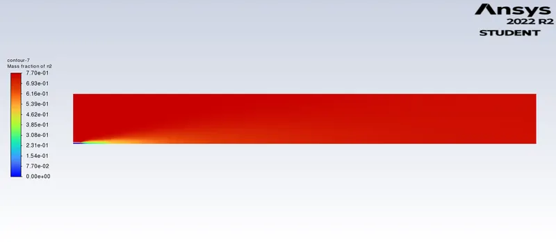
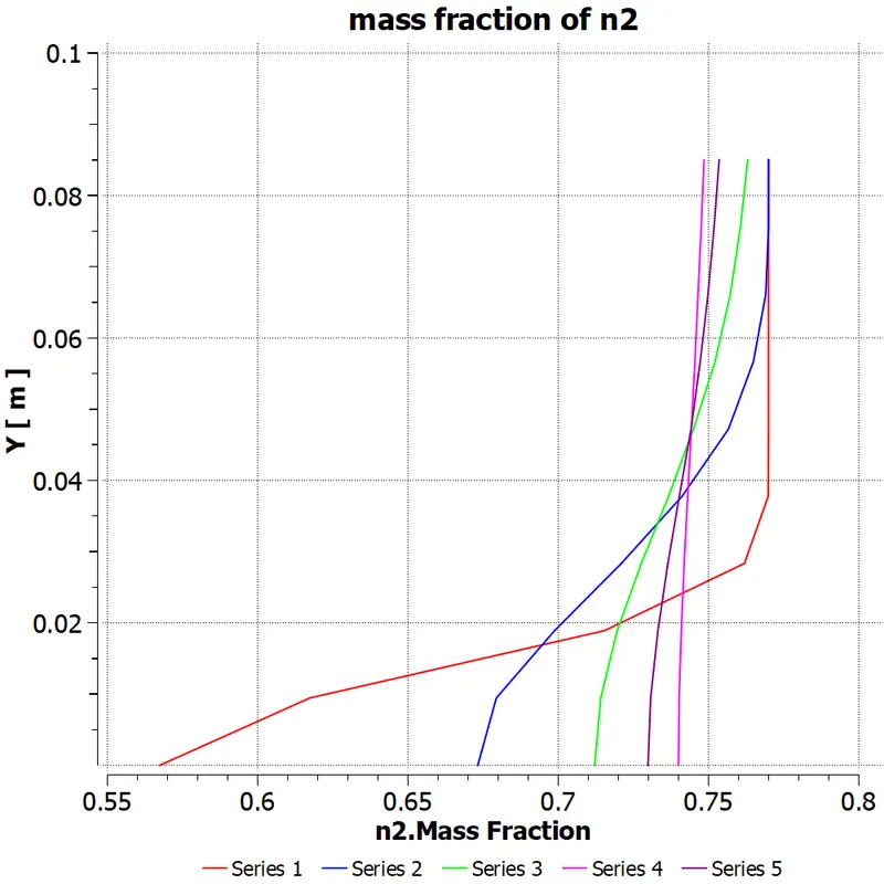
5.Mass Fraction Of N2

6.Mass fraction of O2

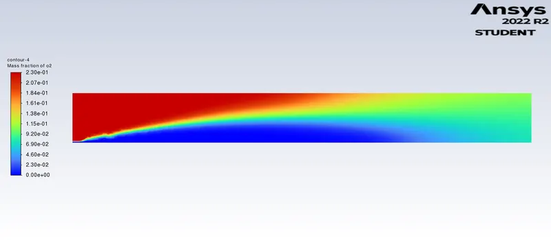
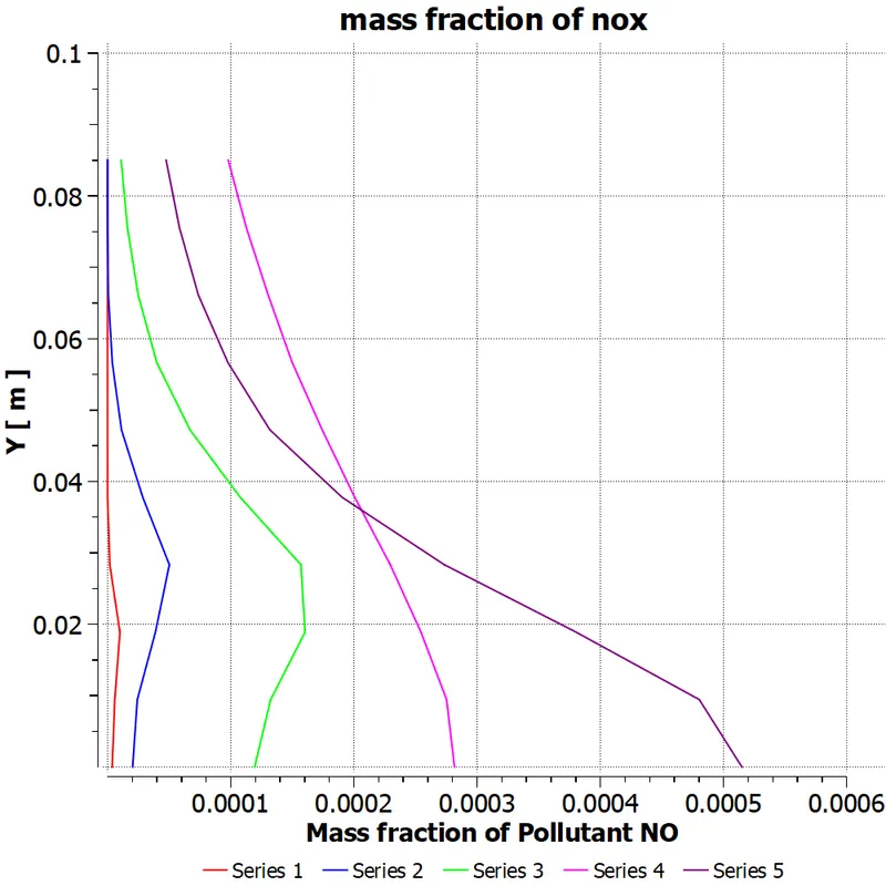
7. Mass fraction of NOx

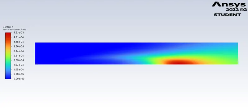
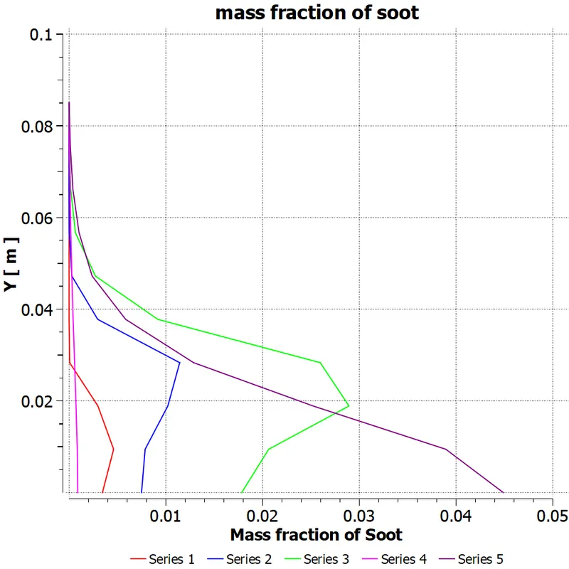
8.Mass fraction of soot formation

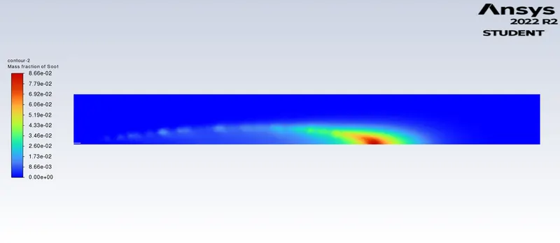
9.Temperature obtained during the simulation

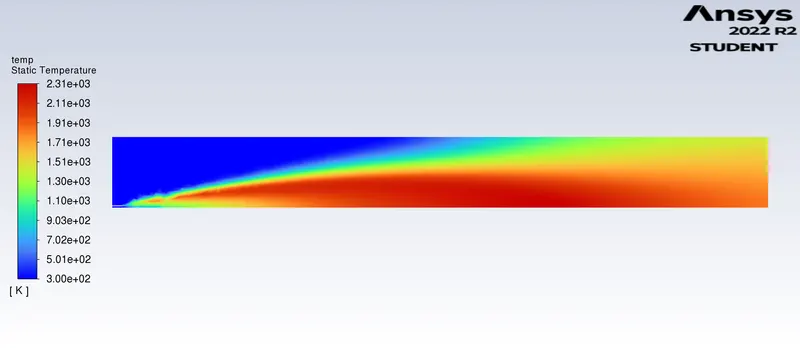
Chart Showing Variation of different species using line probes

1. Chart of Mass fraction of CH4

2.Chart of Mass Fraction of CO2

3. Chart of Mass fraction of H2O

4.Chart of mass fraction of N2

5.Chart of Mass fraction of O2

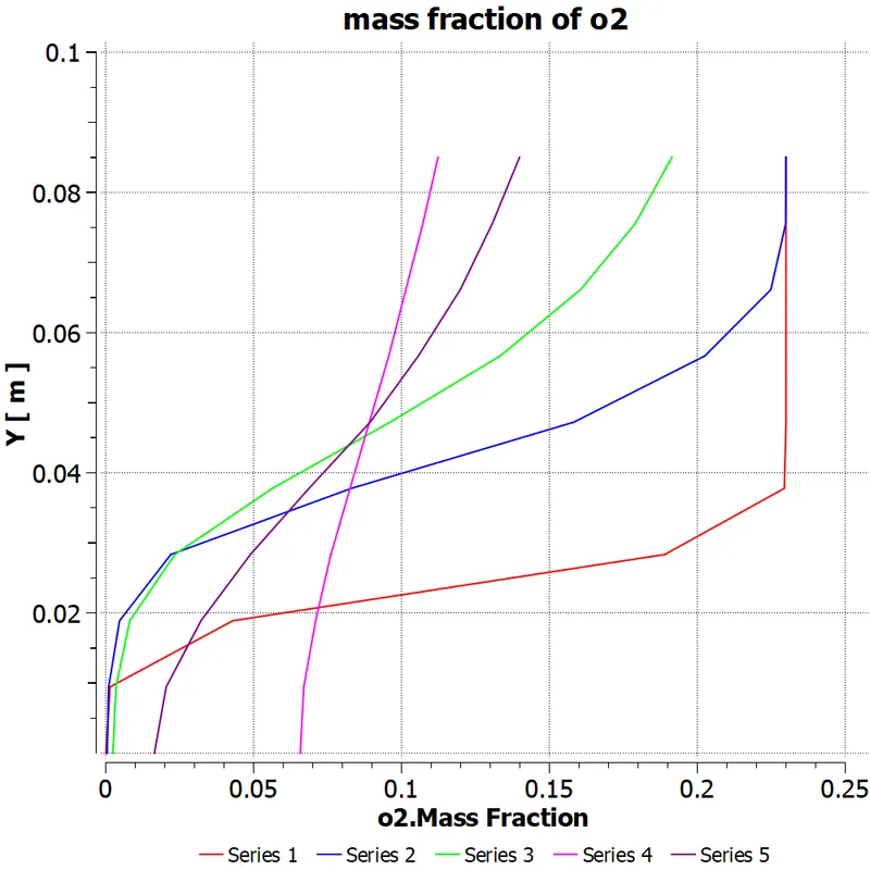
6. Chart of Mass fraction of NOx

7. Chart of Mass Fraction of soot

Part II -

In this part, We add the water content in the fuel from 5% to 30% by mole and observe the effect of it on the results. We provide line plots and contours to prove our claim.We use the parametric study approach for this part.

• As you must have observed from the above simulation, the Nox and soot is getting formed at the outlet of the combustor. Such formation has harmful effects on the environment and humans. The stringent government norms also demand the least formation of Nox and soot and to satisfy those requirements,we need to check the effect of adding the water in the fuel.
• In this part, we will add the water content in the fuel from 5% to 30% by mole and observe the effect of it on the results and we also provide line plots and contours to prove your claim. We use the parametric study approach for this part.So let us start by setting up simulation.
• Everything is same as previous case from the point of geometry and mesh.
• Comming to set up the change comes here .As we are performing parametric study we need to set input parameters and output parameters to perform the parametric study.
• We need to keep water and CH4 mass fraction as input parameters and want to moniter the temperature and emmisions ( NOx and soot ) at the outlet .So , we keep area weighted average of them as output parameters.
• To parametrize the mass fractions of water(H2O) and CH4 input parameters we have to follow below steps,

steps : while giving bounday conditions to fuel inlet , under species mass fractions instead of giving values for mass fractions ,click on the side options of CH4 and select new input parameter->then name it -> click ok .

• In the same way set mass fractions of H2O as new input parameter and for remaining all species give zero (0) .
• To parametrize temperature and emmisions ( NOx and soot ) as output parameter we have to follow below steps,

steps : solution -> under definitions -> select new -> select the surface report ->area weighted average-> and select the filed variable as temepreature and at surfaces we select outlet-> check report file and report plot ->and to parametrize the mass flow rate we need to select/mark the output parameter -> then okay.

• In the similar way we also create report for NOx and soot formation at the outlet and select/mark the output parameter.This creates area weighted average of NOx and soot formation as output parameter.
• In the same way you can also parametrize other quantities if needed.
• Remaining everything is same as previous case.
• Now if you close the fluent and go back to workbench you will observe a new option has added ie., parameters.
• If you double click on it you will find a new tab is opened as shown in the below image.

Fig:- Parametrization of the water and fuel mixture for observing the NOx and Soot formation

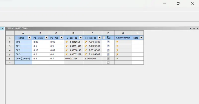
• We create 4 design point with water content in the fuel from 5% to 30%(mass fractions for water(H2O)as 0 , 0.05 ,0.15, 0.25, 0.3) as there is already one design point with water percent 0 .
• To view the updated geometry ,meshing ,solution data ,animations ,contours etc. of newly created design point you need to click on the retain data.
• Now we need to update all the design point by clicking on the update all design points.
• After updating the design points you will observe the values of temperature and emmisions ( NOx and soot ) in the output column for all the created design points.
• Then after that we can see the individual solution date by right click on the name of design point and selecting set as current.Then we can go to workbench and view the result of the required design point.
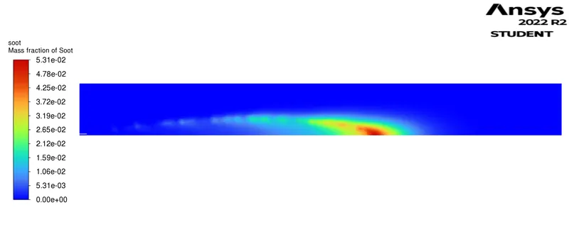
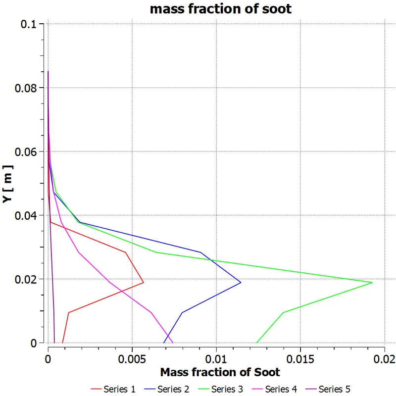
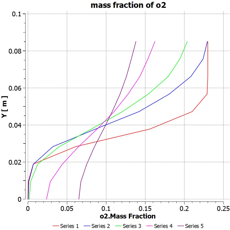
  • Now let us plot the contour of temperature distribution , mass fraction of NOx and soot and also Chart showing variation of the mass fraction of soot and NOx along Y-direction at different locations (along X-axis) of the combustor for all the cases and then conclude by observing the effect of addition of water on results.

Case-1:- Water Content in the Fuel = 5%

Plots , Contours and Charts of mass fraction obtained from this simulation are:-

1.Residuals

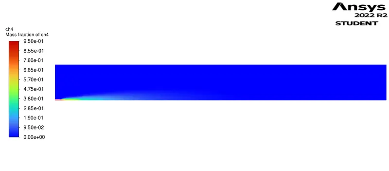
2. Mass fraction of CH4

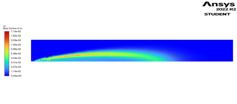
3.Mass fraction of CO

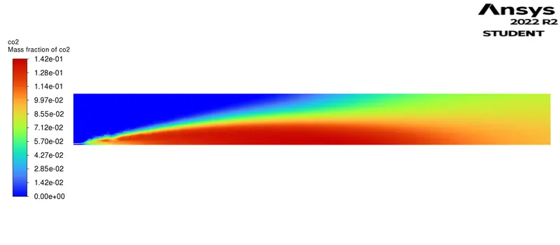
4.Mass fraction of CO2

5. Mass fraction of H20

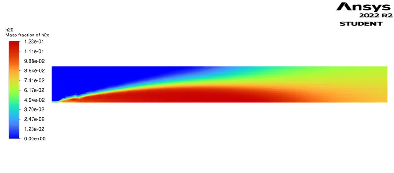
6.Mass fraction of N2

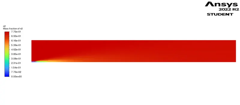
7.Mass fraction of o2

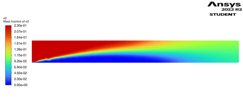
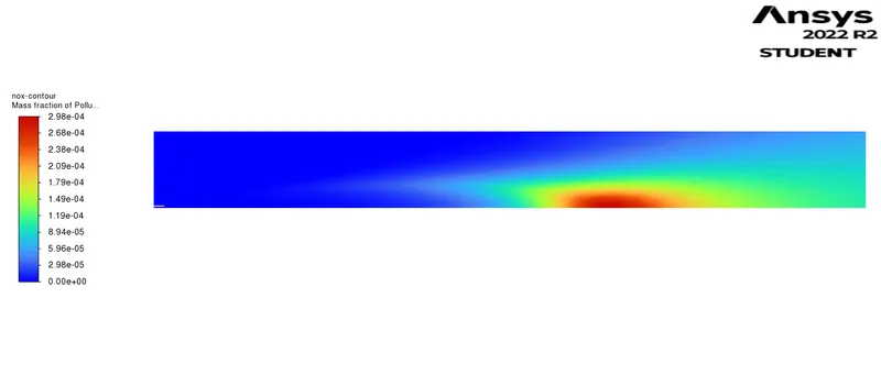
8. Mass fraction of Nox

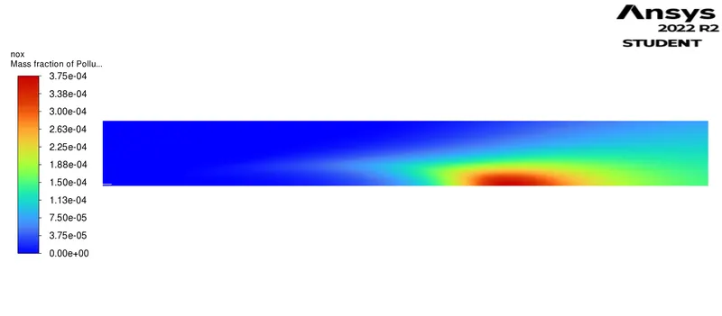
9.Mass fraction of soot

10.Temperature Contour

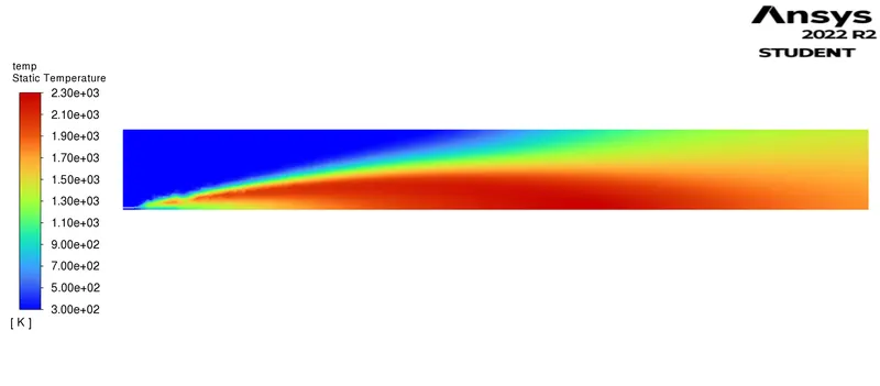
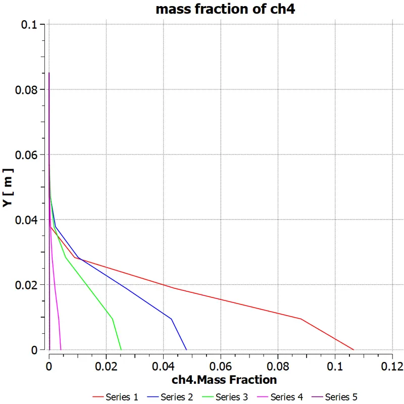
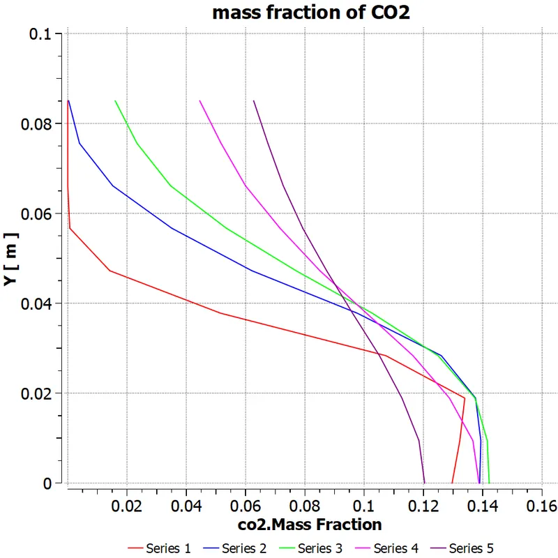
Chart of Mass Fractions

1. Chart of CH4

2. Chart of CO2

3. Chart of CO

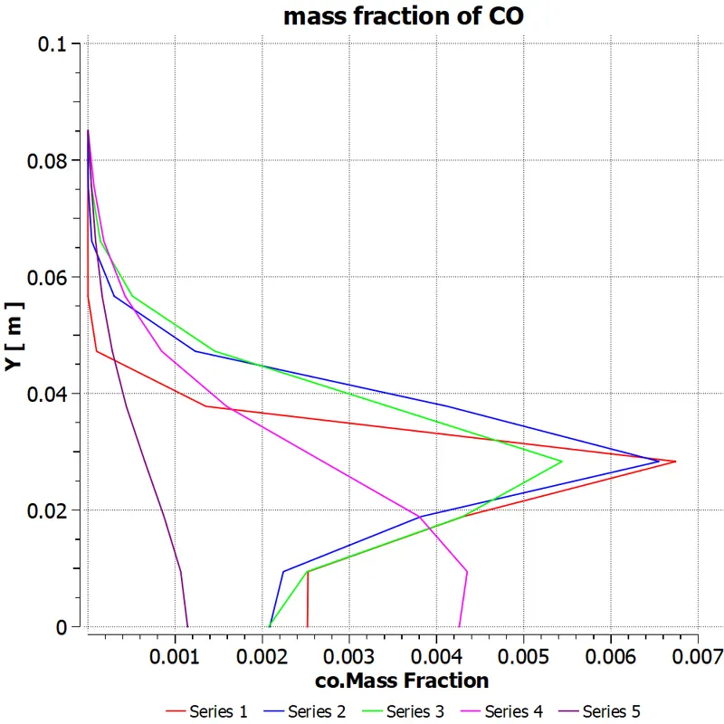
4.Chart of N2

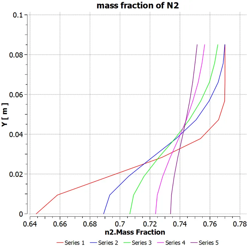
5. Chart of O2

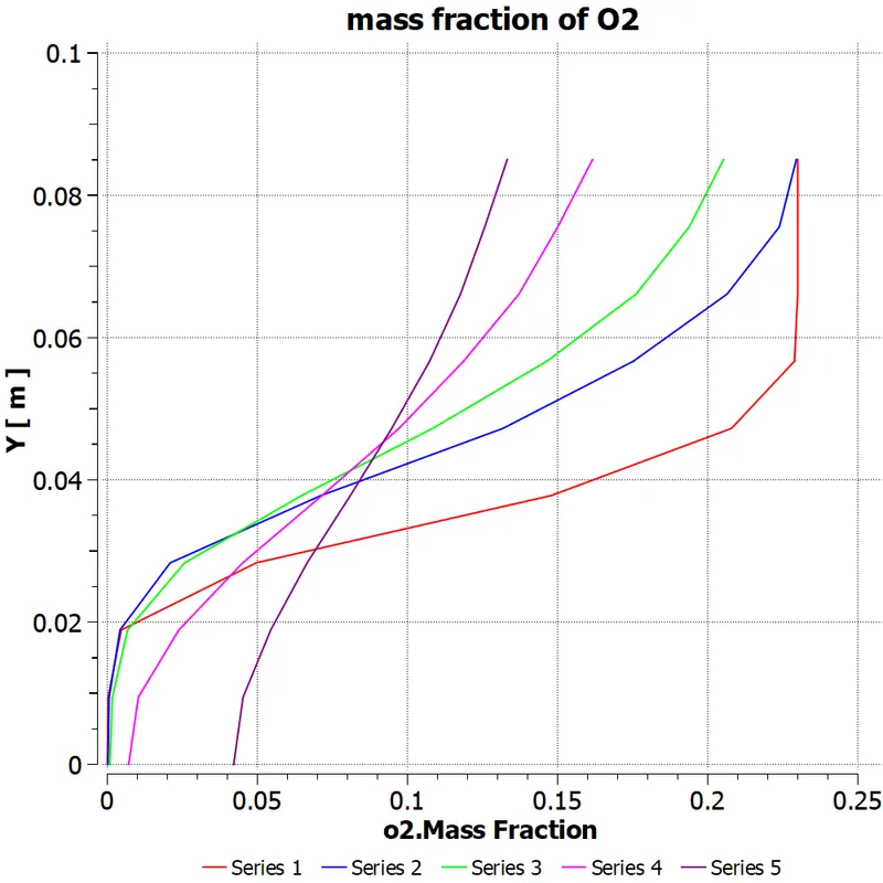
6. Chart of H2O

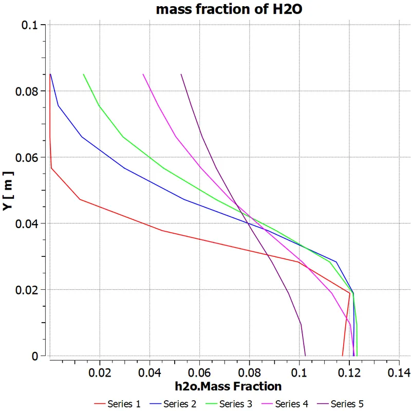
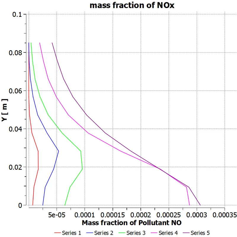
7. Chart of NOx

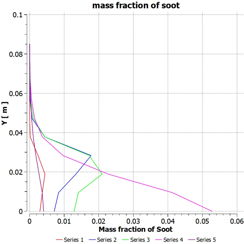
8. Chart of soot

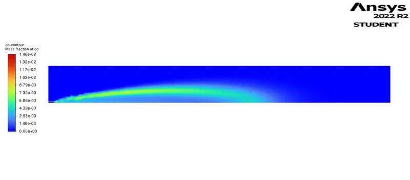
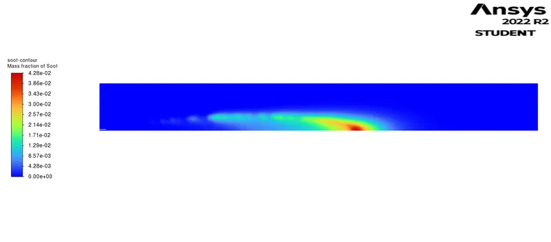
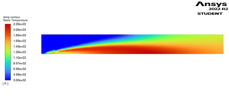
Case-2 :- Water content in the fuel = 10%

Plots , Contours and charts obtained from this simulation are:-

1. Residuals

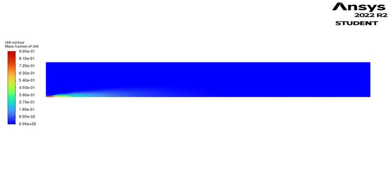
2. Mass fraction of CH4

3.Mass fraction of CO2

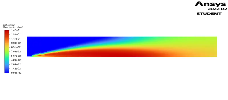
4.Mass fraction of N2

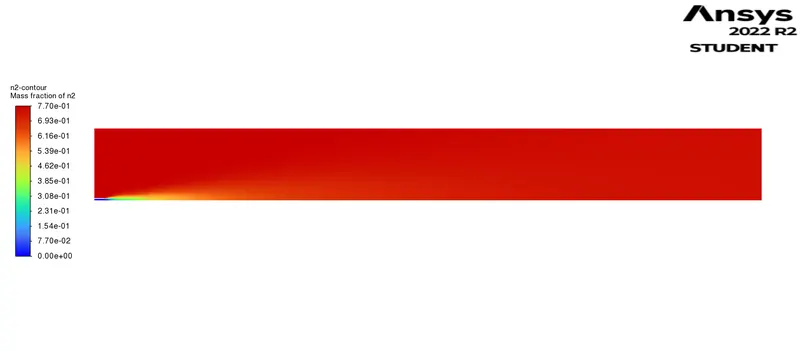
5.Mass Fraction of O2

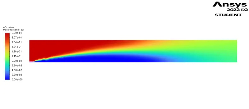
6.Mass Fraction of H2O

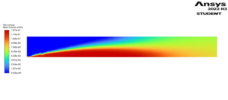
7.Mass fraction of CO

8.Mass fraction of NOx

9.Mass fraction of soot

10.Temperature Contour

Charts of Mass fractions

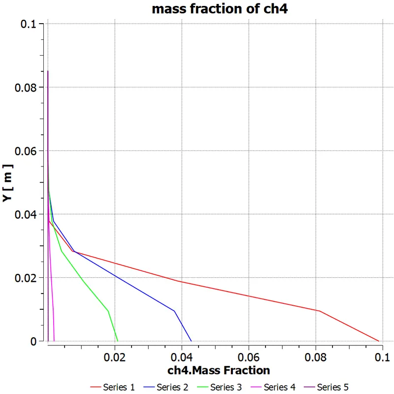
1. Chart of CH4

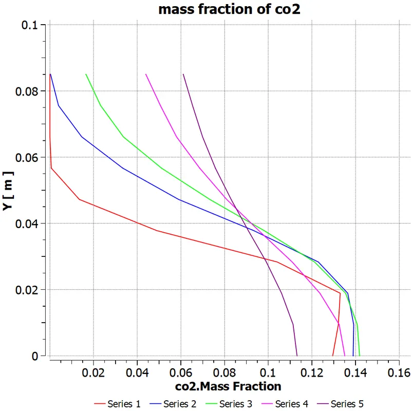
2.Chart of CO2

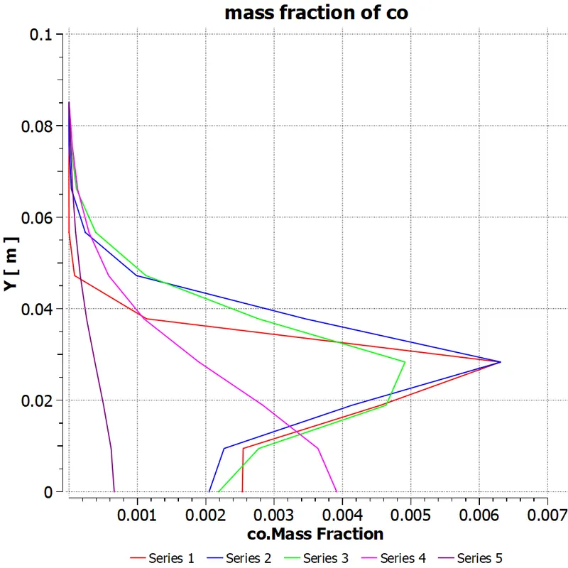
3.Chart of CO

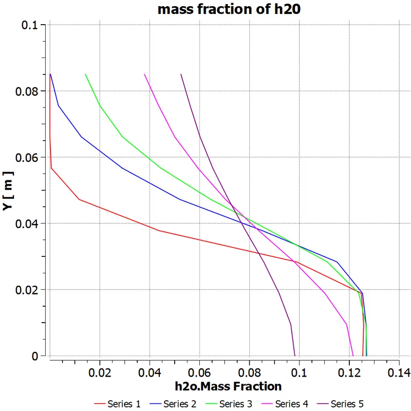
4.Chart of H20

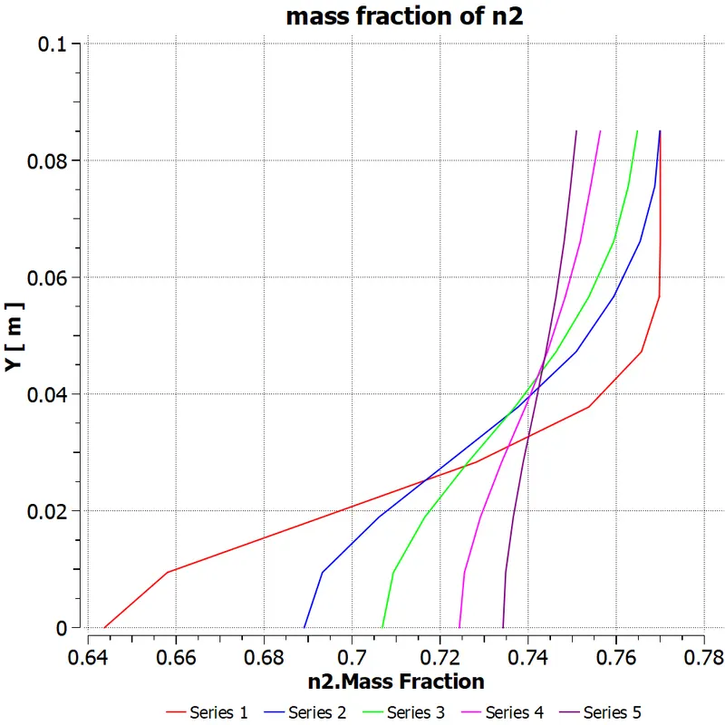
5.Chart of N2

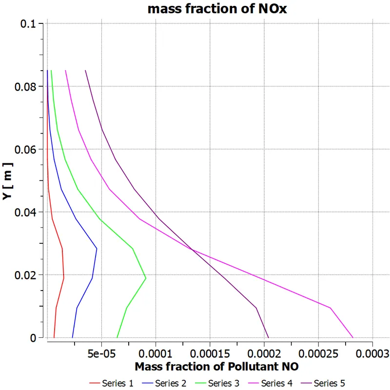
6.Chart of NOx

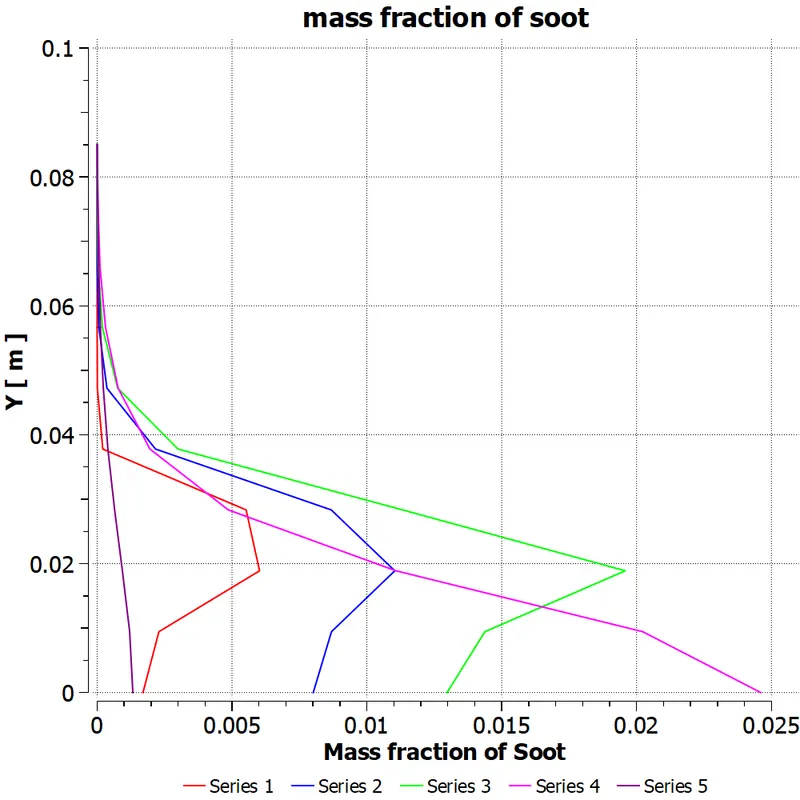
7.Chart of Soot

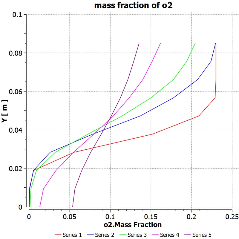
8.Chart of O2

Case-3 :- Water content in the Fuel = 15%

Plots , Contours and Charts obtained

Mass Fraction of the species

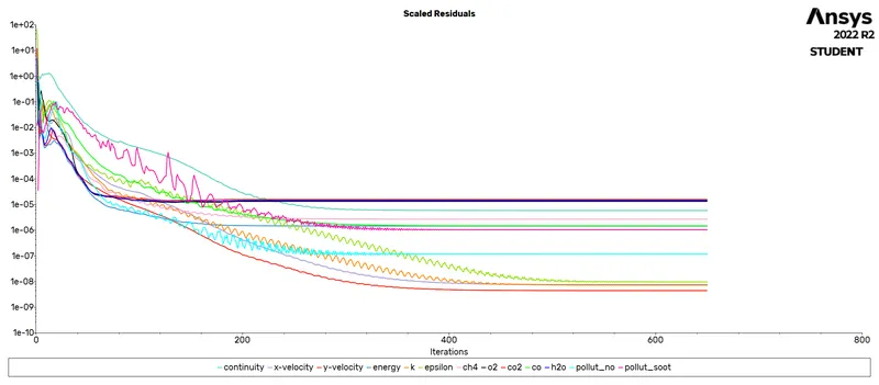
1.Residuals

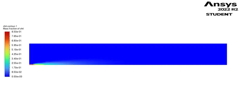
2. Mass fraction of CH4

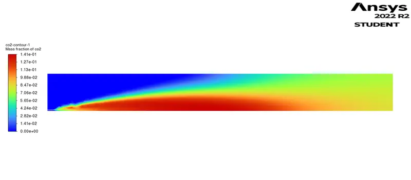
3. Mass fraction of CO2

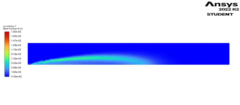
4. Mass fraction of CO

5.Mass fraction of H2O

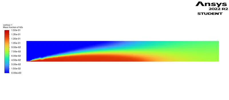
6.Mass fraction of O2

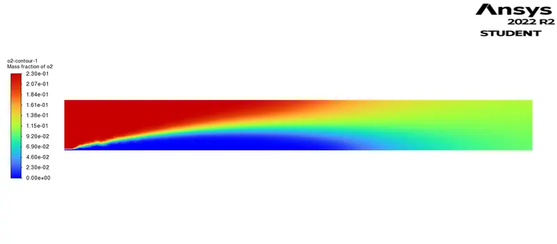
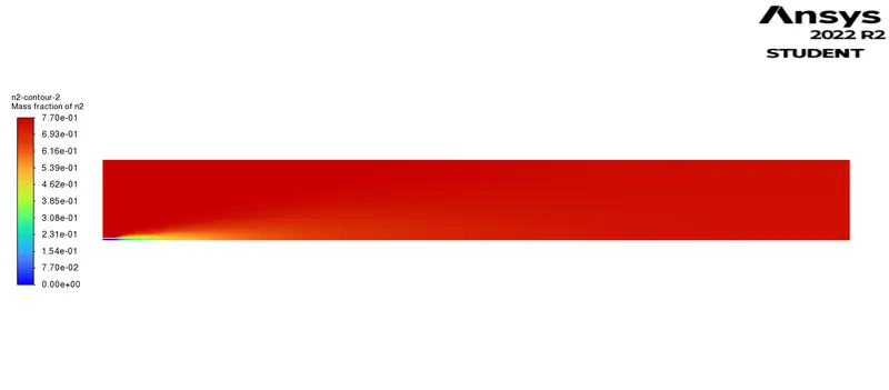
7. Mass fraction of N2

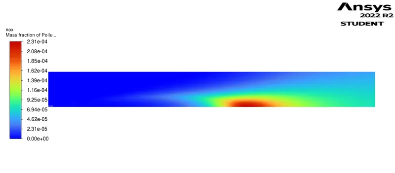
8. Mass fraction of NOx

9. Mass fraction of soot

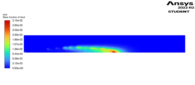
10. Temperature Contour

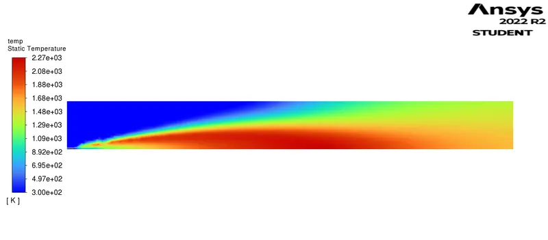
Charts of the Mass fraction of the species

1.Chart of CH4

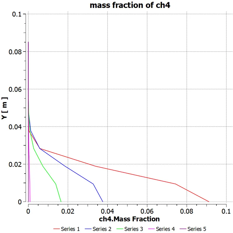
2. Chart of CO

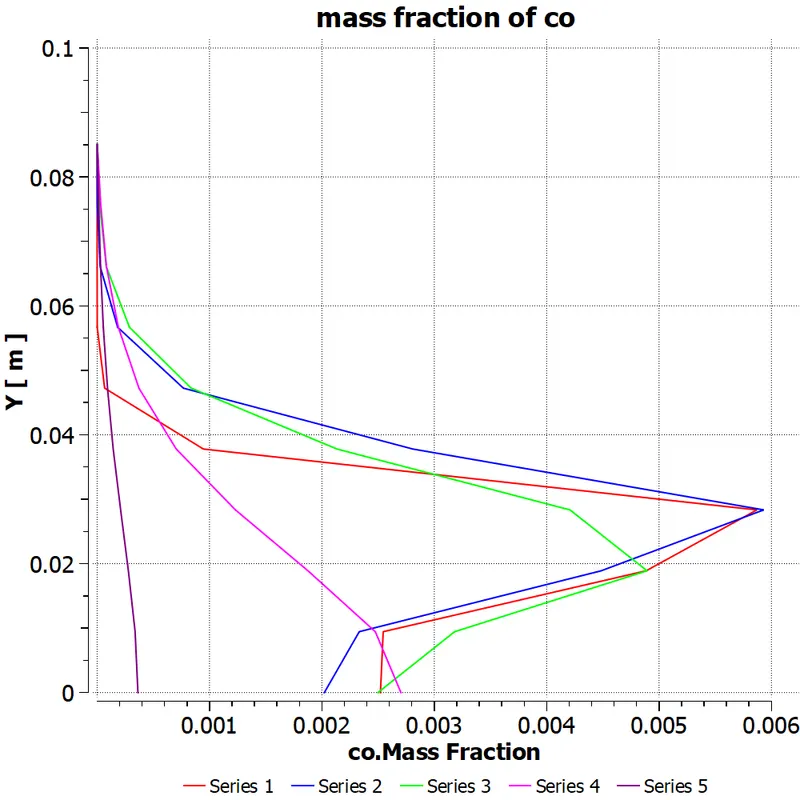
3.Chart of CO2

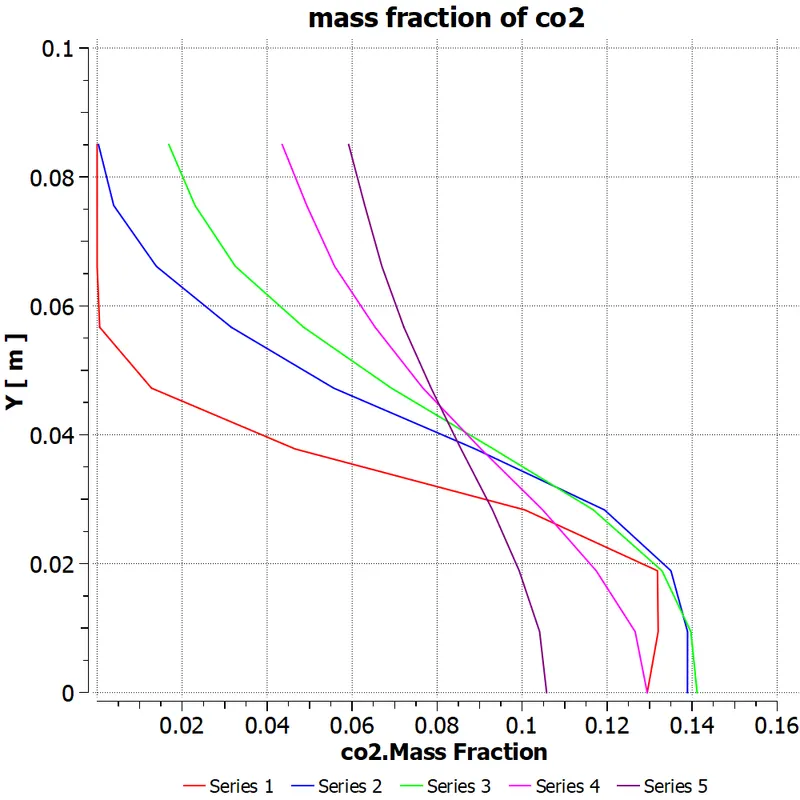
4.Chart of H2O

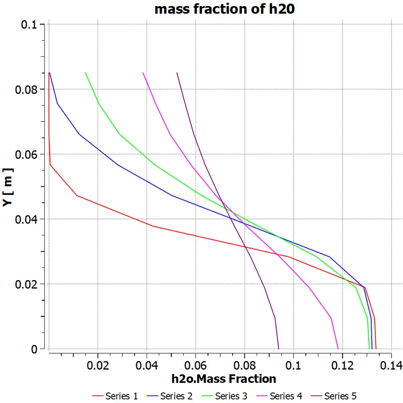
5.Chart of N2

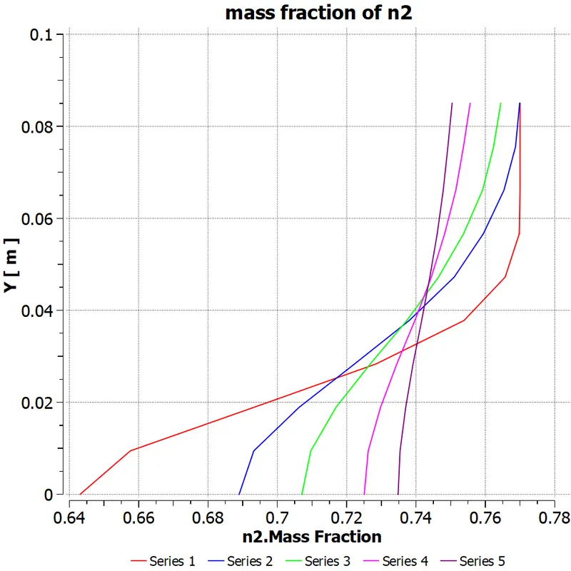
6.Chart of NOx

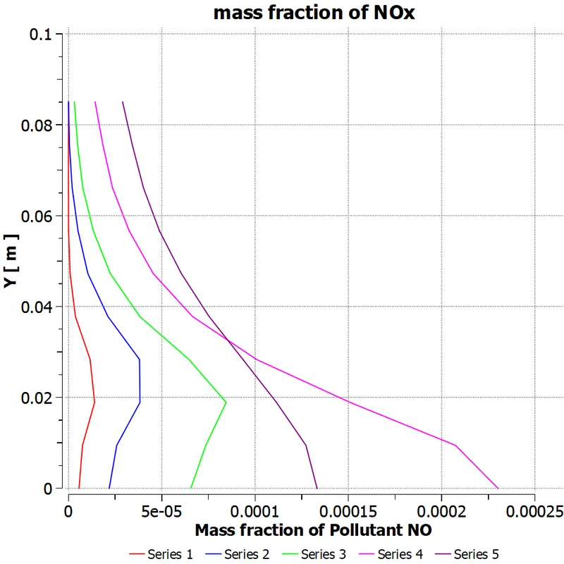
7. Chart of soot

8.Chart of O2

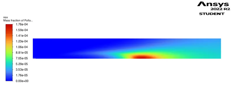
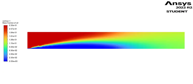
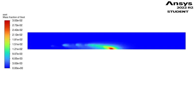
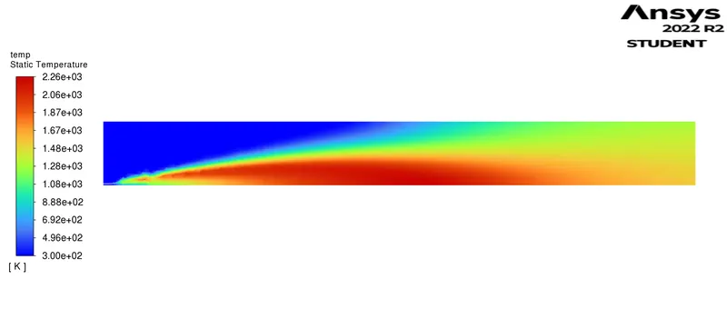
Case-4:- Water content in the Fuel = 20%

Plots , Contours and Charts obtained are

Mass Fraction of the species are:-

1. Residuals

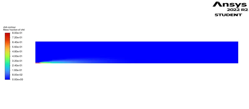
2. CH4

3.CO2

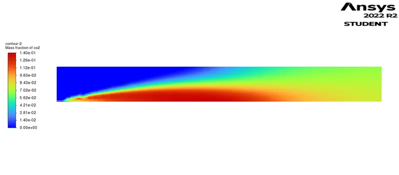
4.CO

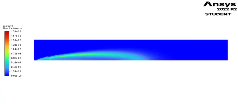
5.H2O

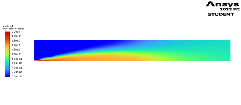
6.N2

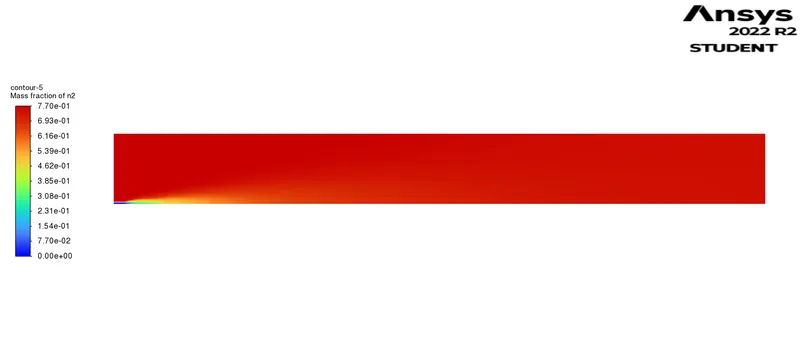
7.NOx

8.O2

9.soot

10.temperature

Charts of the mass fraction of the species are:-

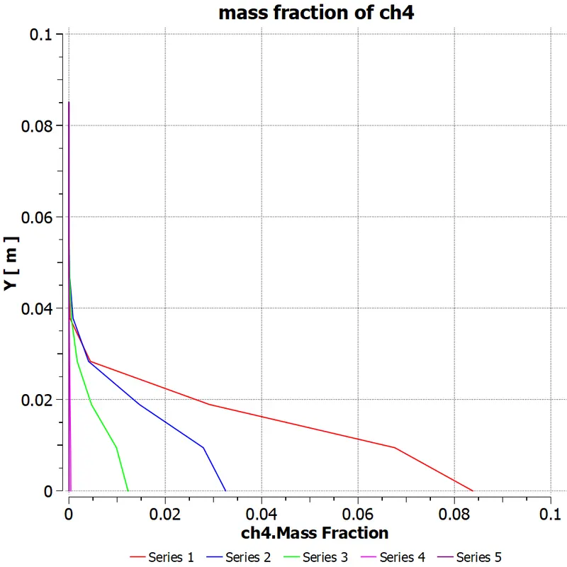
1.CH4

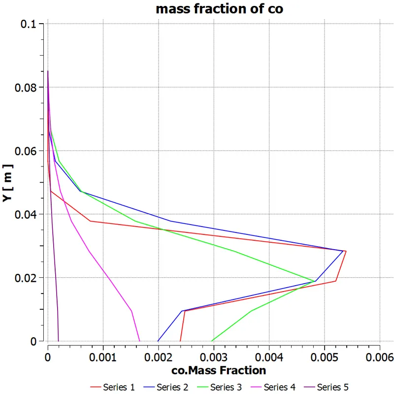
2.CO

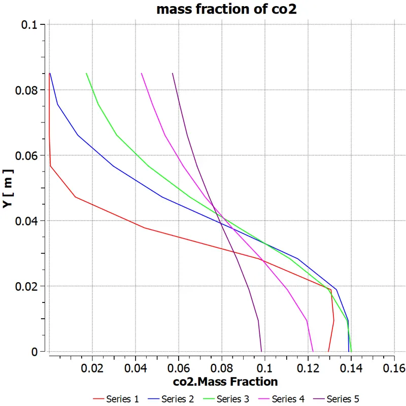
3.CO2

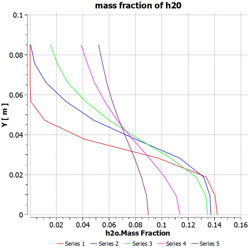
4.H2O

5.N2

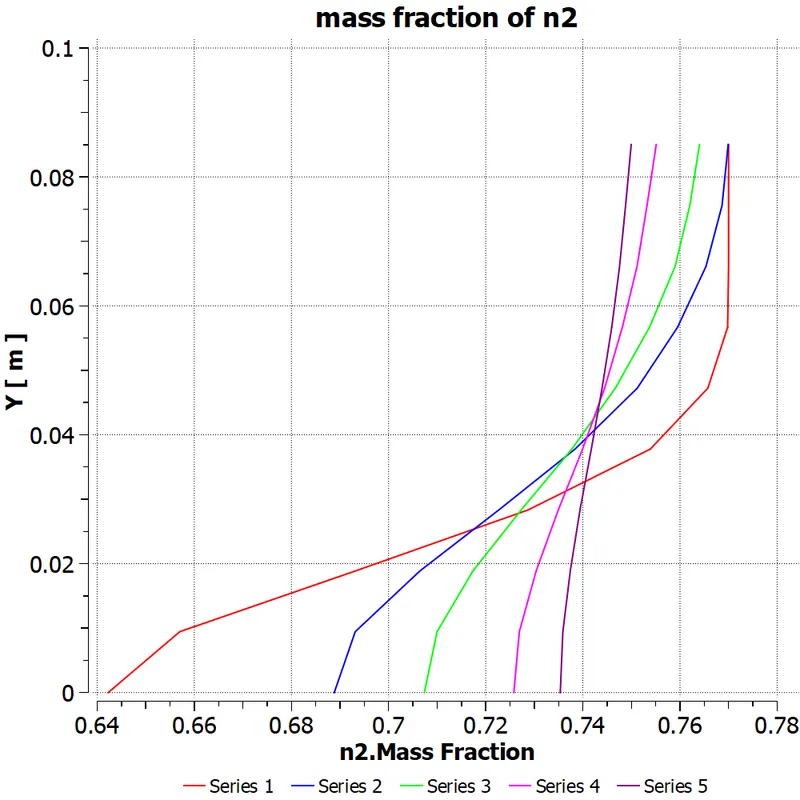
6.NOx

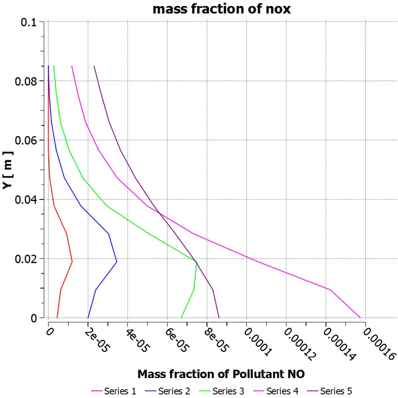
7.o2

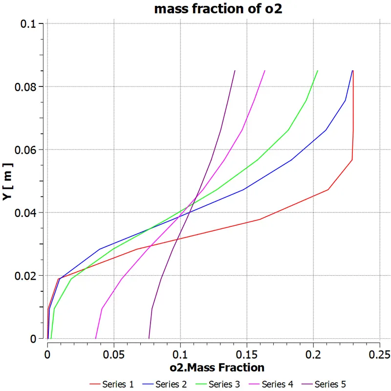
8.soot

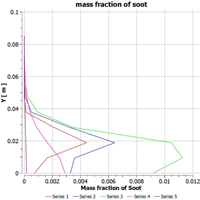
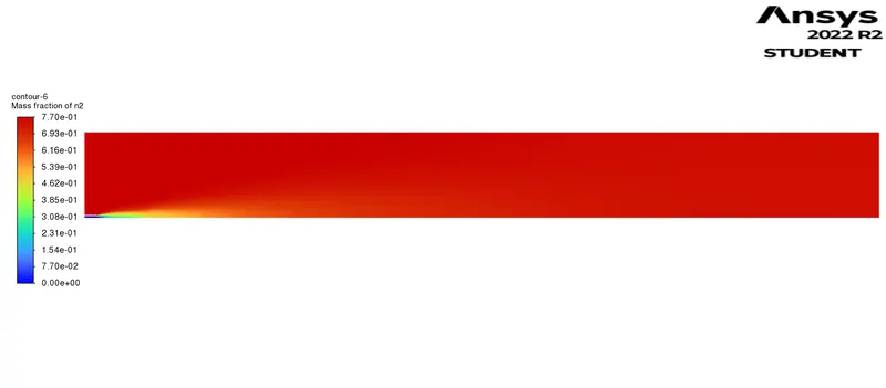
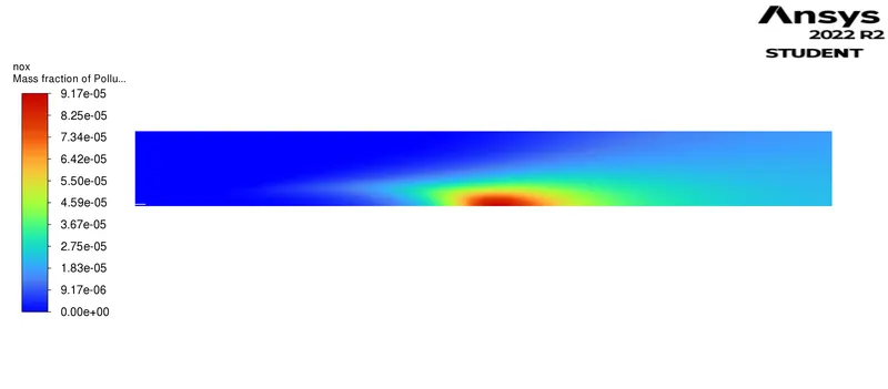
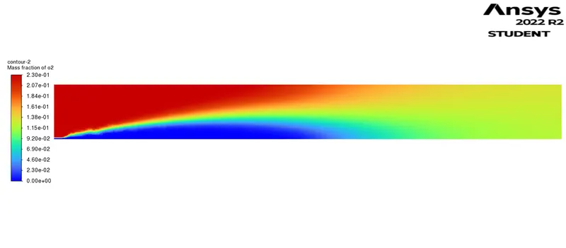
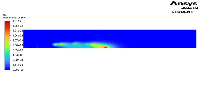
Case-5:- Water Content in the Fuel = 30%

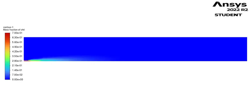
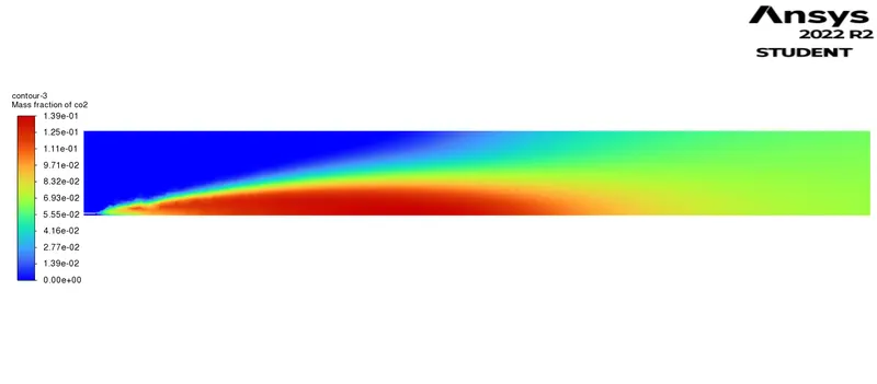
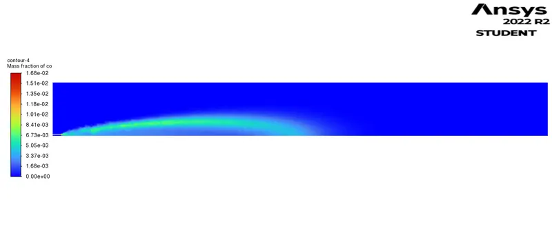
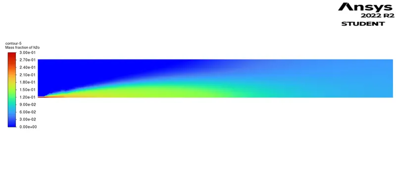
Plots , Contours and Charts obtained from the simulations are:-

Mass fraction of the species are:-

1.CH4

2.CO2

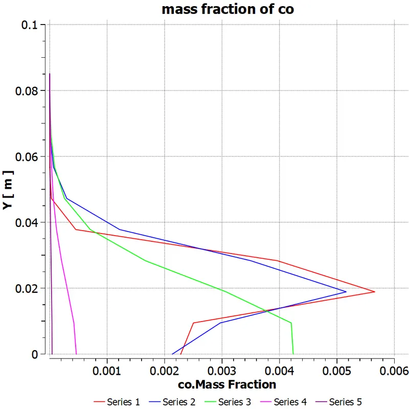
3.CO

4.H2O

5.N2

6.NOx

7.O2

8.soot

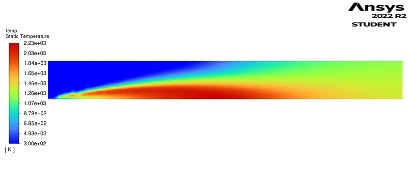
9.temperature

10.Residuals

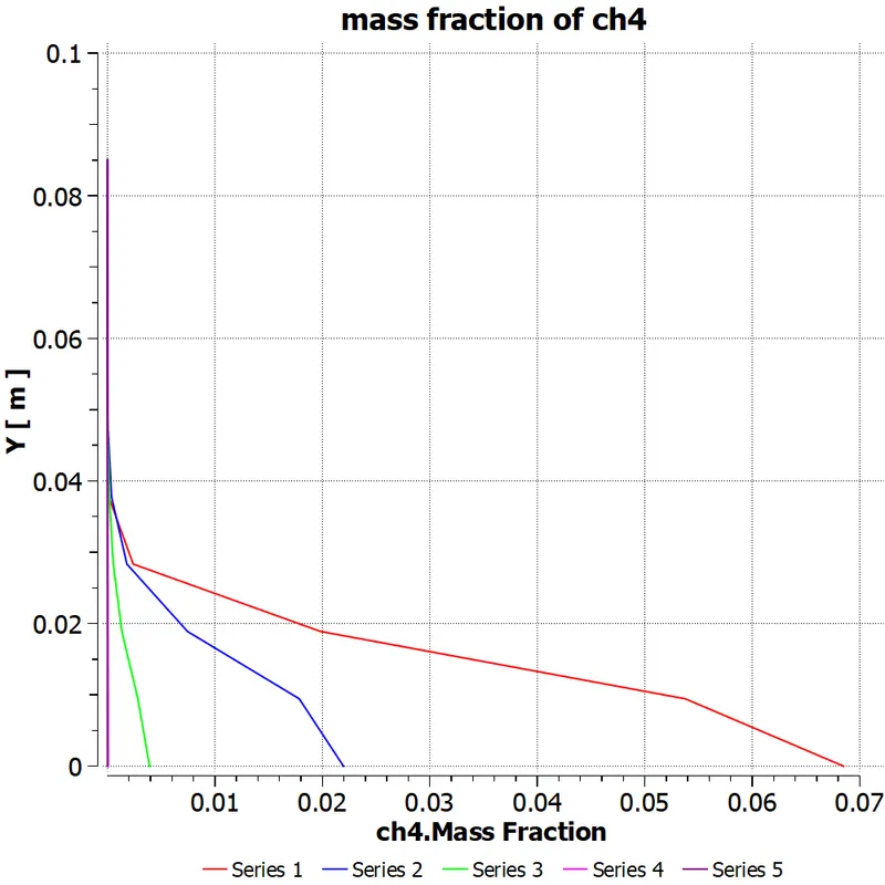
charts of the Mass fraction of the species

1.CH4

2.CO

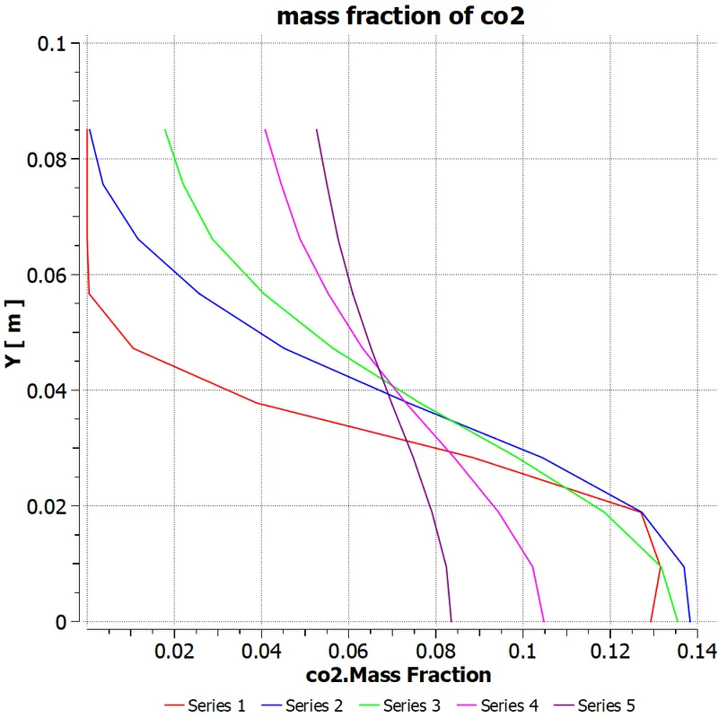
3.CO2

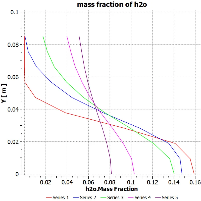
4.H2O

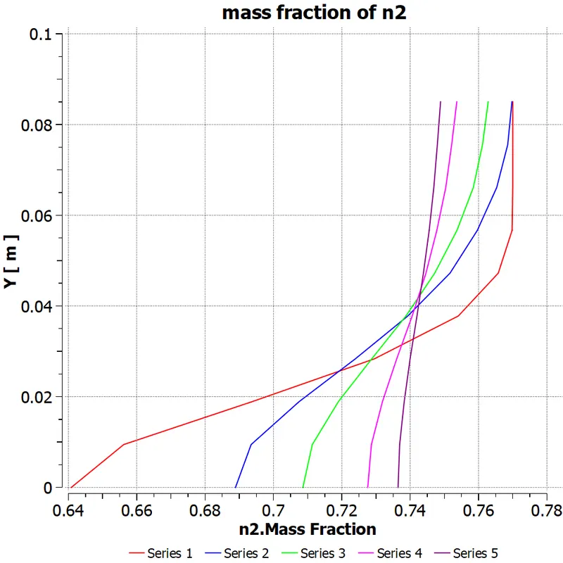
5.N2

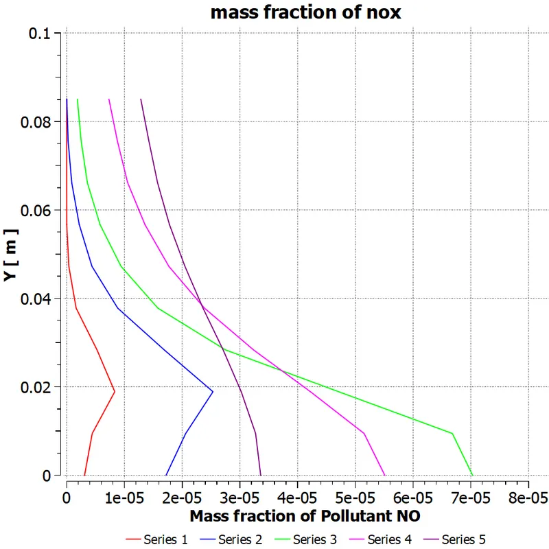
6.NOx

7.O2

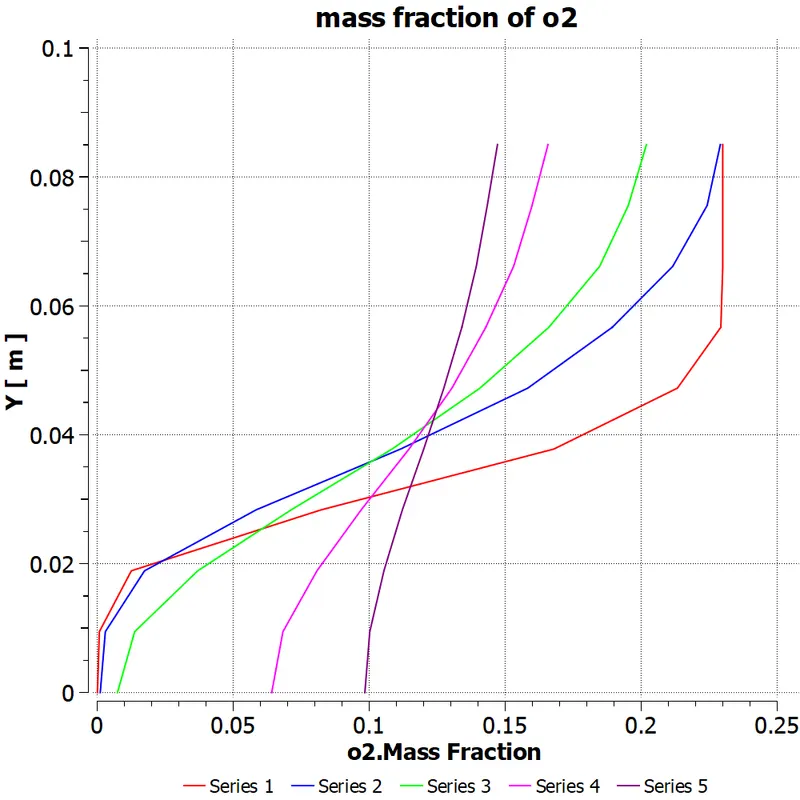
8.soot

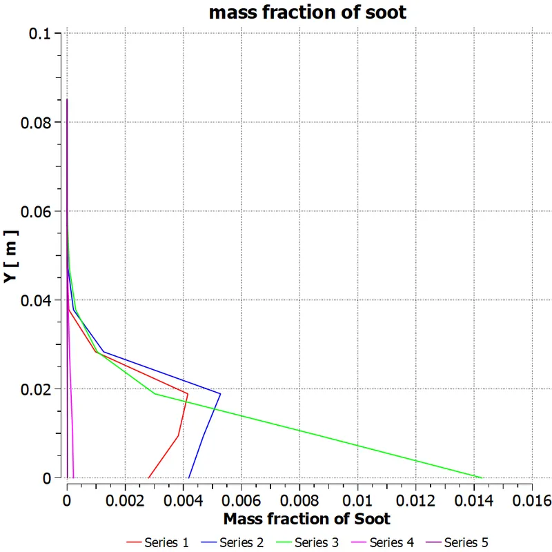
CONCLUSIONS:-

Impact of adding water to the fuel:

We can now say that the emissions (creation of Nox and soot) have been at their lowest when adding water to the fuel based on the parametric chart or the above contours and charts. We can see that in case 1 the emissions are fairly high in comparison to case 5, where there has been a greater input of water. Therefore the more water added, the less emissions there will be, but you should also notice that the maximum temperature at the outlet is dropping, which reduces efficiency (if it is a burner). Finally, we can say that by blending water with fuel, emissions have been reduced.

However, the combustion would not be as proper if you added additional water. Thus, the quantity of water added should be raised so that emissions are managed in accordance with established regulatory standards.