Proportional Valve simulation
AIM
The aim of this simulation is to capture flow characteristics of proportional valve
OBJECTIVES
- Variation of lift of valve
- Comparison of results with and without AMR
- FSI model integration with transient case solver
PROPORTIOAL VALVE
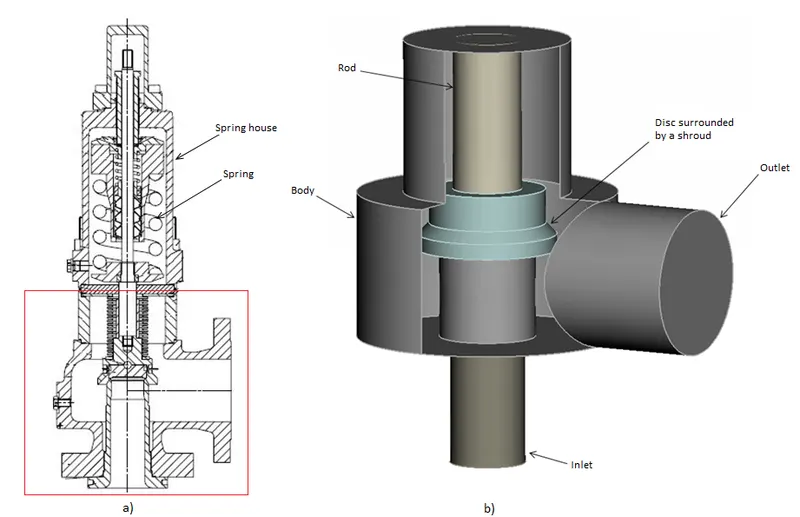
The valve body of a safety relief valve is typically designed with an angle of 90 between the inlet and outlet connections. The valve inlet connection, or nozzle, is mounted on the pressure-containing system and the outlet is usually connected to a piped discharge system. However, in some applications, such as compressed air systems, the safety relief valve will not have an outlet connection, and the gas is vented directly to the atmosphere. The disc is the main part of the valve which is moving in order to regulate the pressure in the system. The valve inlet and the disc are the only parts of the safety relief valve which are exposed to the process uid during normal operating condition, i.e. when the valve is closed. During this condition the disc is held against the seat on the inlet by a spring, which is housed in a spring housing arrangement mounted on top of the body. The spring is connected to the disc by a rod, and the amount of compression the spring is able to maintain is usually adjusted with a spring adjuster in order to alter the pressure at which the disc is lifted o its seat. Discs which are used in rapid opening safety relief valves are often surrounded by a shroud which helps to create the rapid opening of the valve [1]. Usually the disc, shroud and rod are together called spindle. Figure shows the drawing which was used when creating the geometry of the safety relief valve.
A proportional valve provides a change in output pressure or flow in the same ratio as the change in the input, for example if the input doubles then the output will also double. Proportional valves can be interconnected with the output from one being used as the input to another.
Increasing the current increases the strength of the magnetic field and, in turn, the force of attraction (or repulsion) on the magnetic material. A proportional valve has a geometry to ensure a constant field strength, at a given current, over the stroke of the magnet.
Also, a spring is introduced to counter the force of the magnet; as the spring is compressed by movement of the magnet, the spring reaction force increases until it balances the magnetic force and movement ceases. If the current is increased, the magnet (solenoid) moves further against the spring, until the forces are balanced again. Consider that the magnet is attached to a spool in a valve, the pressure or flow can be controlled in proportion to the current applied to the solenoid.
PROPORTIONAL VALVES [ 3 MM LIFT WITHOUT AMR]
Geometry
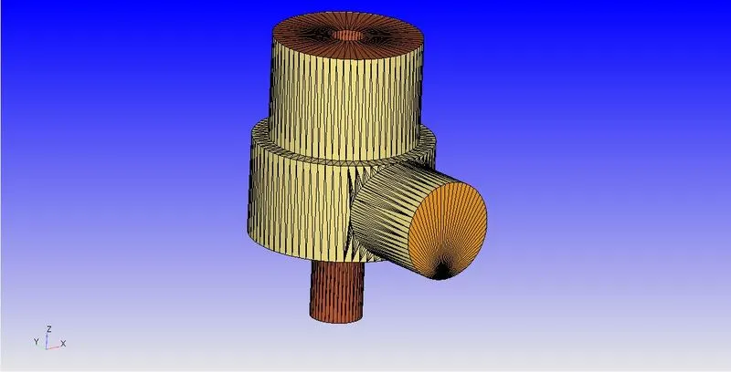
Mesh
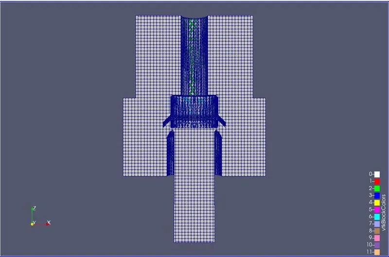
For the mesh size, the default setting of 0.004m size cells were used which takes the cell count to about 80000.
Boundary Conditions
Wall Inlet
- Wall Boundary
- Temperature = 300K
Wall Casing
- Wall Boundary
- Temperature = 300K
Inlet
- Pressure = 30 Bar
- Temperature = 300 K
- Species - Air
Outlet
- Pressure = 1 Bar
- Temperature = 300 K
- Species - Air
Valve Spindle
- Wall Boundary
- Temperature = 300K
Results
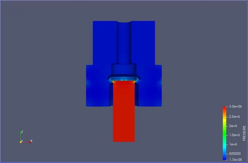
Pressure Contour
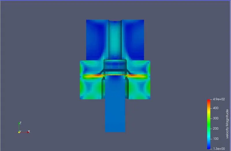
Velocity Contour
Mass Flow Rate Plot
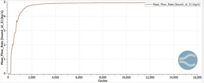
Now for 3 mm lift of the valve, the air rushes through the inlet at rate of 5 kg/s
Velocity Plot
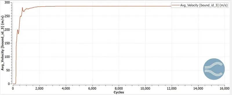
Due to the huge pressure difference we see a large value of velocity of 280 m/s
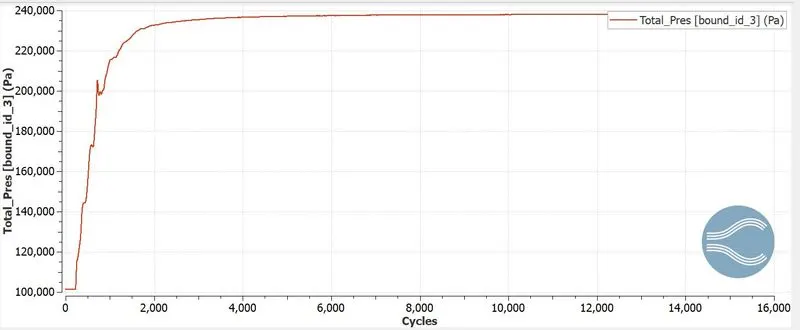
Pressure Plot
Temperature Plot
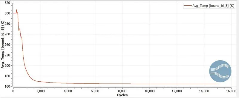
There is a significant loss of temperature of air which drops to 165 K.
Cell Count
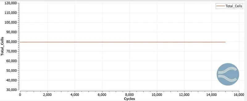
The total cell count has gone upto 80000 cells.
PROPORTIONAL VALVES [ 3 MM LIFT WITH AMR]
Geometry
Mesh
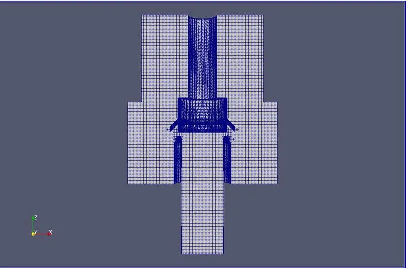
For the mesh size, the default setting of 0.004m size cells were used which takes the cell count to about 100000.
Boundary Conditions
Wall Inlet
- Wall Boundary
- Temperature = 300K
Wall Casing
- Wall Boundary
- Temperature = 300K
Inlet
- Pressure = 30 Bar
- Temperature = 300 K
- Species - Air
Outlet
- Pressure = 1 Bar
- Temperature = 300 K
- Species - Air
Valve Spindle
- Wall Boundary
- Temperature = 300K
Results
Pressure Contour
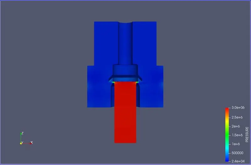
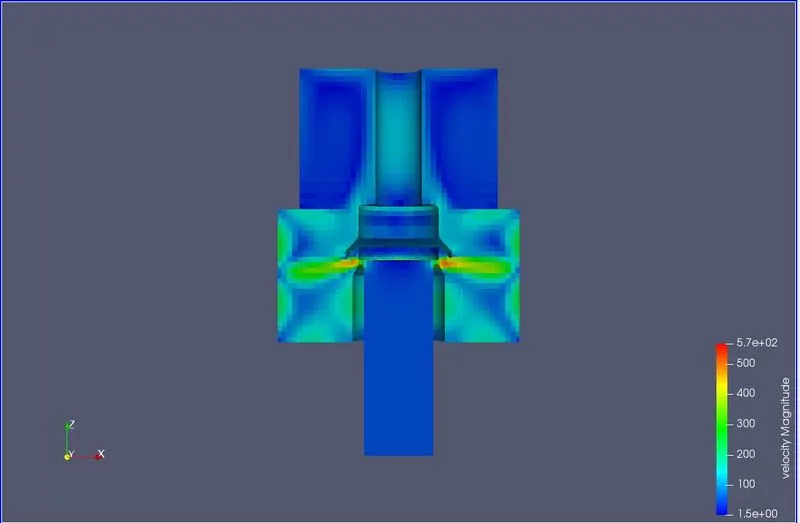
Velocity Contour
Mass Flow Rate Plot
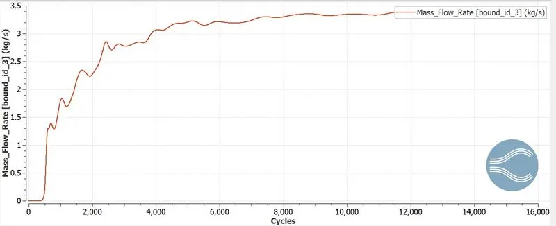
Now for 3 mm lift of the valve, the air rushes through the inlet at rate of 3.4 kg/s
Velocity Plot
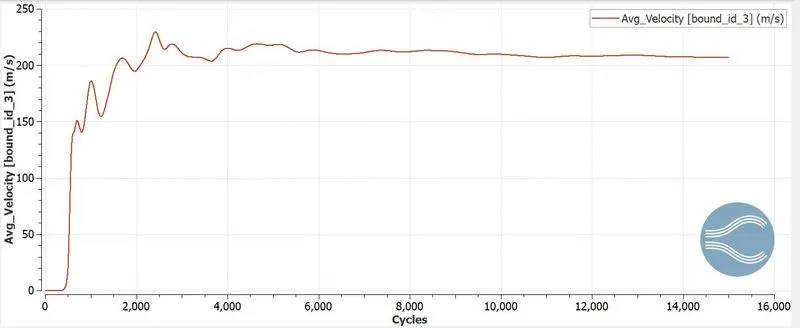
Due to the huge pressure difference we see a large value of velocity of 205 m/s
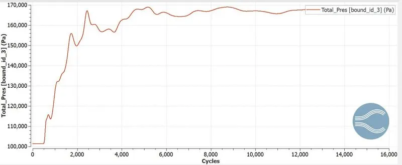
Pressure Plot
Temperature Plot
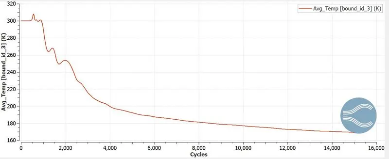
There is a significant loss of temperature of air which drops to 170 K.
Cell Count
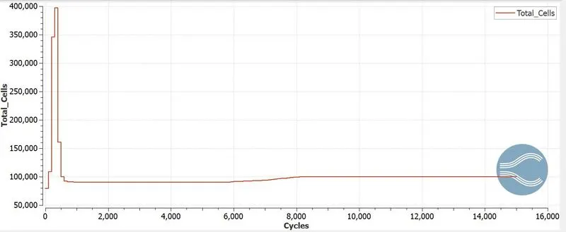
The total cell count has gone upto 100000 cells.
Animation Files of 3 mm lift
PROPORTIONAL VALVES [ 4 MM LIFT WITHOUT AMR]
Geometry
Mesh
For the mesh size, the default setting of 0.004m size cells were used which takes the cell count to about 80000.
Boundary Conditions
Wall Inlet
- Wall Boundary
- Temperature = 300K
Wall Casing
- Wall Boundary
- Temperature = 300K
Inlet
- Pressure = 30 Bar
- Temperature = 300 K
- Species - Air
Outlet
- Pressure = 1 Bar
- Temperature = 300 K
- Species - Air
Valve Spindle
- Wall Boundary
- Temperature = 300K
Results
Pressure Contour
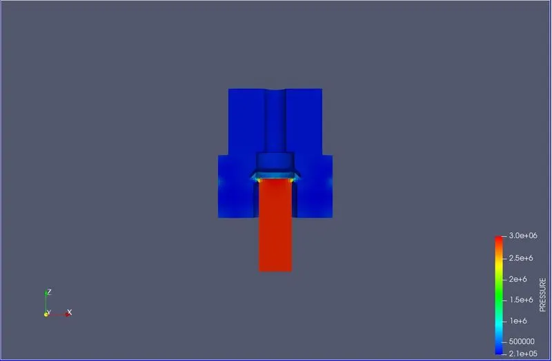
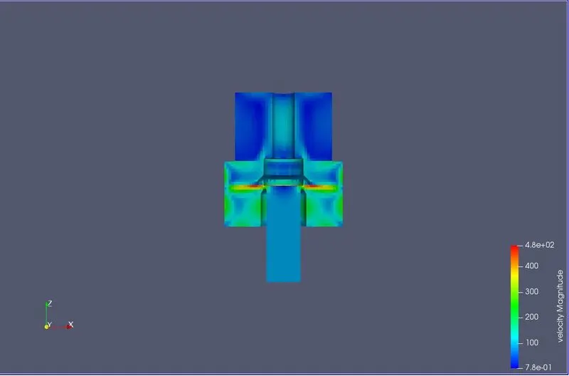
Velocity Contour
Mass Flow Rate Plot
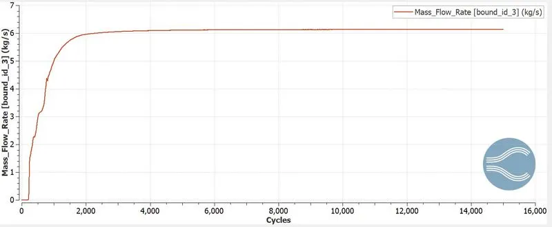
Now for 4 mm lift of the valve, the air rushes through the inlet at rate of 6 kg/s
Velocity Plot
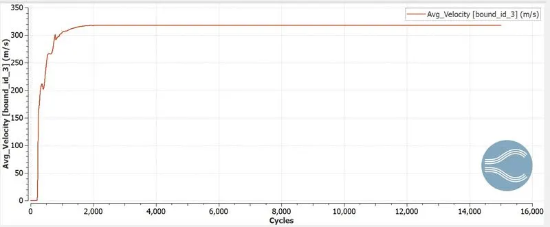
Due to the huge pressure difference we see a large value of velocity of 320 m/s
Pressure Plot
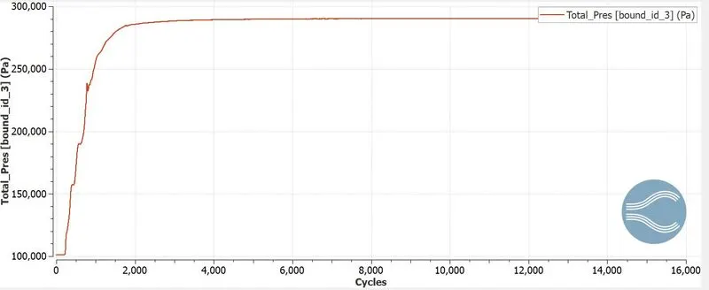
Temperature Plot
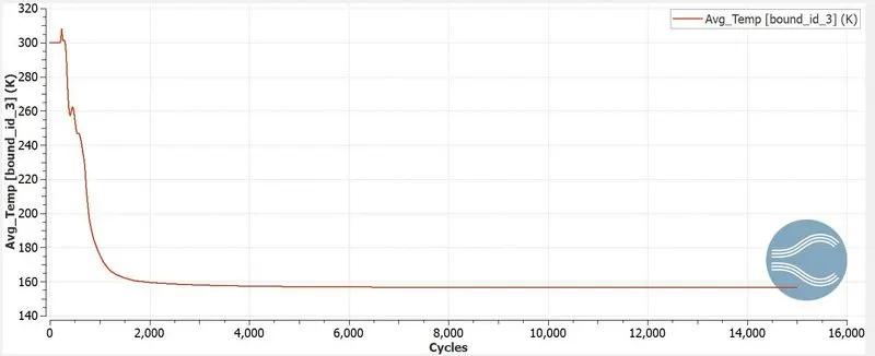
There is a significant loss of temperature of air which drops to 160 K.
Cell Count
The total cell count has gone upto 80000 cells.
PROPORTIONAL VALVES [ 4 MM LIFT WITH AMR]
Geometry
Mesh
For the mesh size, the default setting of 0.004m size cells were used which takes the cell count to about 80000.
Boundary Conditions
Wall Inlet
- Wall Boundary
- Temperature = 300K
Wall Casing
- Wall Boundary
- Temperature = 300K
Inlet
- Pressure = 30 Bar
- Temperature = 300 K
- Species - Air
Outlet
- Pressure = 1 Bar
- Temperature = 300 K
- Species - Air
Valve Spindle
- Wall Boundary
- Temperature = 300K
Results
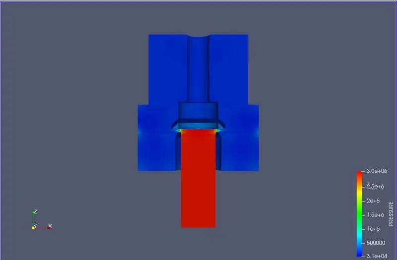
Pressure Contour
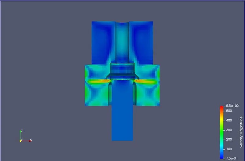
Velocity Contour
Mass Flow Rate Plot
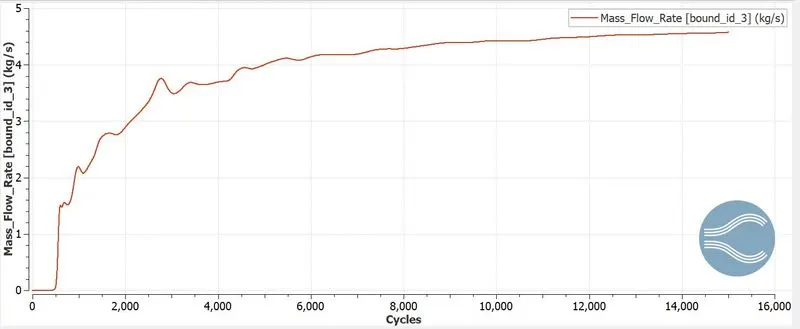
Now for 4 mm lift of the valve, the air rushes through the inlet at rate of 4.5 kg/s
Velocity Plot
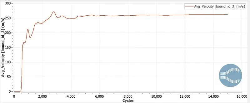
Due to the huge pressure difference we see a large value of velocity of 260 m/s
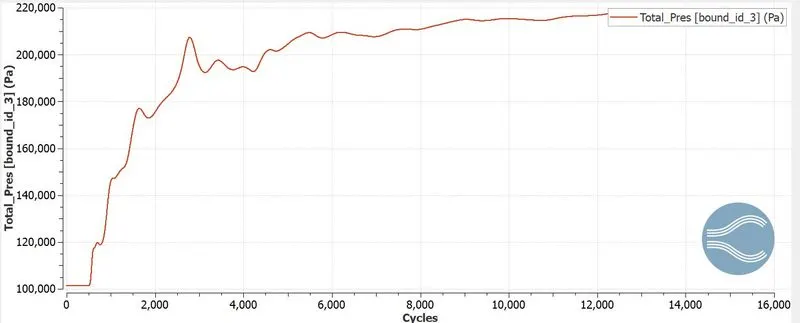
Pressure Plot
Temperature Plot
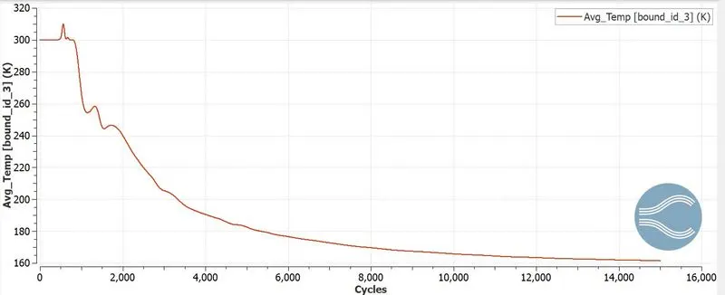
There is a significant loss of temperature of air which drops to 160 K.
Cell Count
The total cell count has gone upto 100000 cells.
Animation for 4 mm lift
PROPORTIONAL VALVES [ 5 MM LIFT WITHOUT AMR]
Geometry
Mesh
For the mesh size, the default setting of 0.004m size cells were used which takes the cell count to about 80000.
Boundary Conditions
Wall Inlet
- Wall Boundary
- Temperature = 300K
Wall Casing
- Wall Boundary
- Temperature = 300K
Inlet
- Pressure = 30 Bar
- Temperature = 300 K
- Species - Air
Outlet
- Pressure = 1 Bar
- Temperature = 300 K
- Species - Air
Valve Spindle
- Wall Boundary
- Temperature = 300K
Results
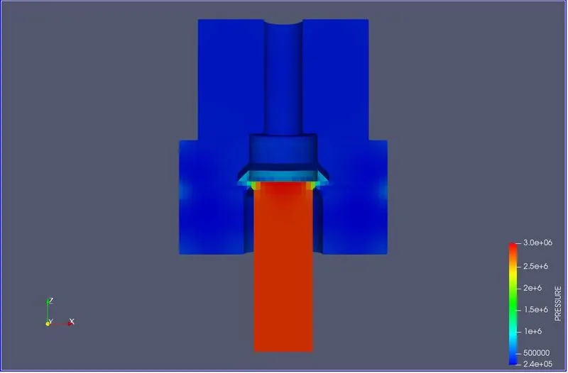
Pressure Contour
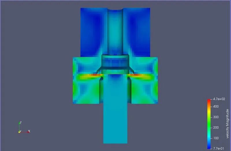
Velocity Contour
Mass Flow Rate Plot
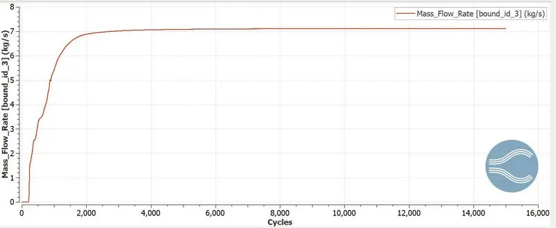
Now for 5 mm lift of the valve, the air rushes through the inlet at rate of 7 kg/s
Velocity Plot
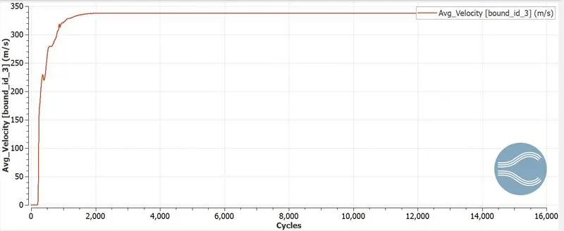
Due to the huge pressure difference we see a large value of velocity of 340 m/s
Pressure Plot
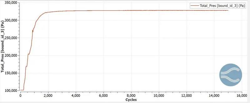
Temperature Plot
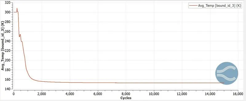
There is a significant loss of temperature of air which drops to 150 K.
Cell Count
The total cell count has gone upto 80000 cells.
PROPORTIONAL VALVES [ 5 MM LIFT WITH AMR]
Geometry
Mesh
For the mesh size, the default setting of 0.004m size cells were used which takes the cell count to about 100000.
Boundary Conditions
Wall Inlet
- Wall Boundary
- Temperature = 300K
Wall Casing
- Wall Boundary
- Temperature = 300K
Inlet
- Pressure = 30 Bar
- Temperature = 300 K
- Species - Air
Outlet
- Pressure = 1 Bar
- Temperature = 300 K
- Species - Air
Valve Spindle
- Wall Boundary
- Temperature = 300K
Results
Pressure Contour
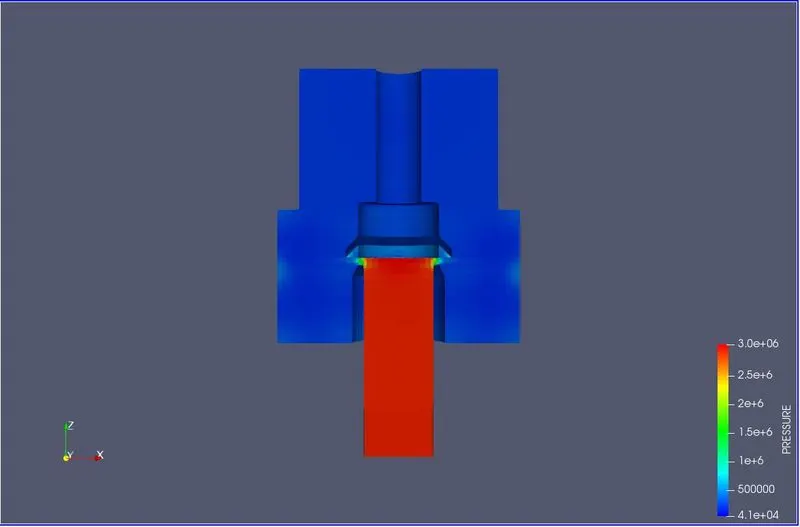
Velocity Contour
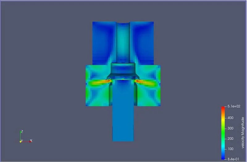
Mass Flow Rate Plot
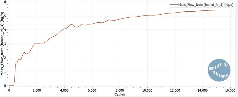
Now for 5 mm lift of the valve, the air rushes through the inlet at rate of 5.5 kg/s
Velocity Plot
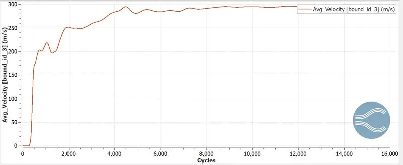
Due to the huge pressure difference we see a large value of velocity of 290 m/s
Pressure Plot
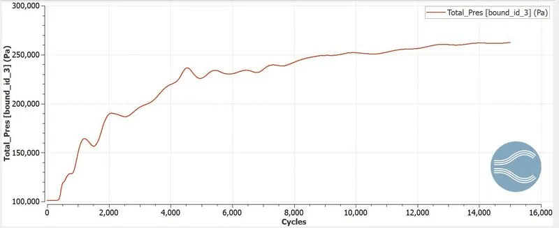
Temperature Plot
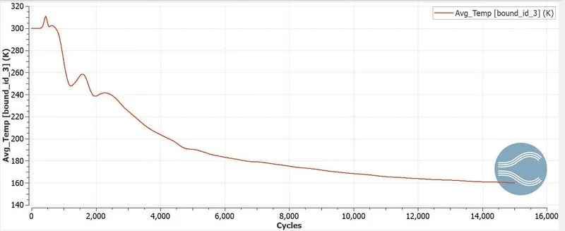
There is a significant loss of temperature of air which drops to 160 K.
Cell Count
The total cell count has gone upto 100000 cells.
Animation for 5 mm lift
PROPORTIONAL VALVE FSI CASE
Geometry
Mesh
For the mesh size, the default setting of 0.004m size cells were used which takes the cell count to about 80000.
Boundary Conditions
Wall Inlet
- Wall Boundary
- Temperature = 300K
Wall Casing
- Wall Boundary
- Temperature = 300K
Inlet
- Pressure = 30 Bar
- Temperature = 300 K
- Species - Air
Outlet
- Pressure = 1 Bar
- Temperature = 300 K
- Species - Air
Valve Spindle
- Wall Boundary
- Temperature = 300K
Fluid Structure Interaction
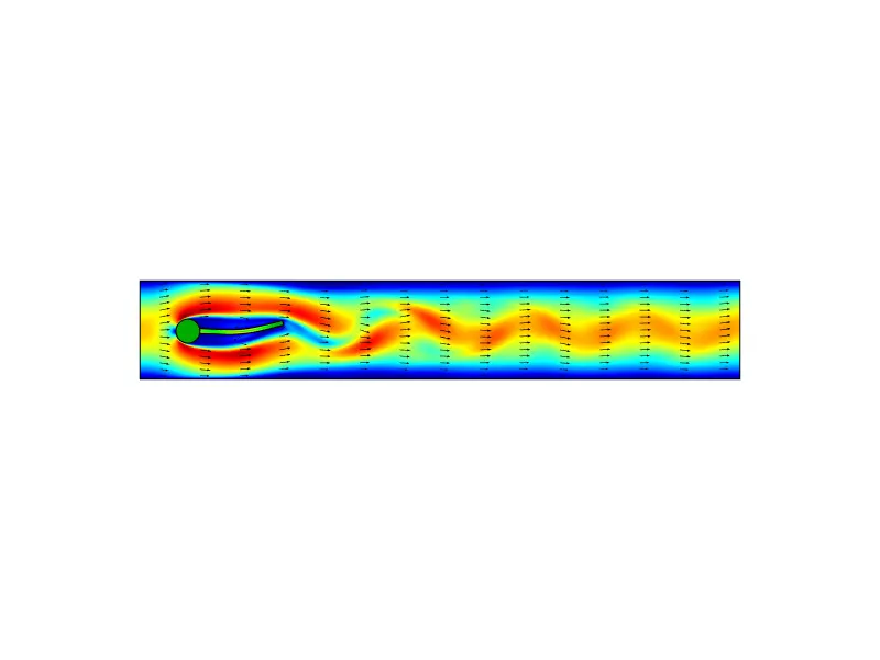
Fluid-structure interaction (FSI) is a multiphysics coupling between the laws that describe fluid dynamics and structural mechanics. This phenomenon is characterized by interactions – which can be stable or oscillatory – between a deformable or moving structure and a surrounding or internal fluid flow.When a fluid flow encounters a structure, stresses and strains are exerted on the solid object – forces that can lead to deformations. These deformations can be quite large or very small, depending on the pressure and velocity of the flow and the material properties of the actual structure.
If the deformations of the structure are quite small and the variations in time are also relatively slow, the fluid's behavior will not be greatly affected by the deformation, and we can concern ourselves with only the resultant stresses in the solid parts. However, if the variations in time are fast, greater than a few cycles per second, then even small structural deformations will lead to pressure waves in the fluid. These pressure waves lead to the radiation of sound from vibrating structures. Such problems can be treated as an acoustic-structure interaction, rather than a fluid-structure interaction.
Yet, if the deformations of the structure are large, the velocity and pressure fields of the fluid will change as a result, and we need to treat the problem as a bidirectionally coupled multiphysics analysis: The fluid flow and pressure fields affect the structural deformations, and the structural deformations affect the flow and pressure.
Results
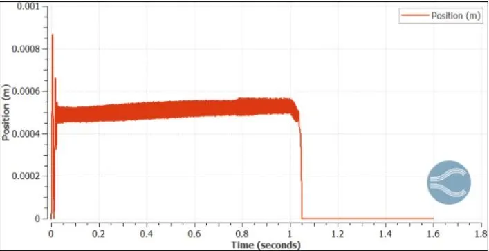
This plot shows the valve spindle position with respect to time, in which it is clearly seen that the amplitude of the lift is alternating. This concept arises due to the fluid first pushing the valve spindle to open, but also one thing should be kept in mind is this valve has spring mass. The spring mass setup will resist the opening and it goes back to the original valve seat. The process continues until 1 second and the spindle just sits back in valve seat according to the pressure condition given in boundary conditions.
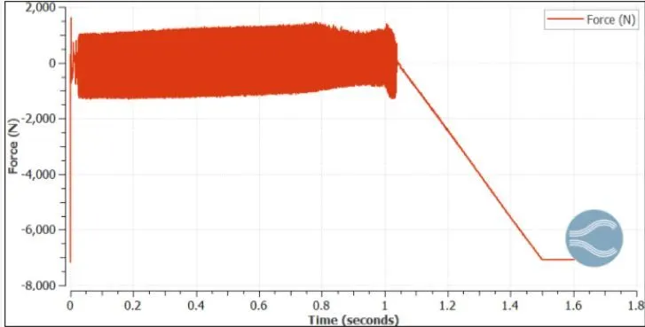
From the force plot we see that the force exerted by the valve spring is 7126 N which was given in the FSI settings, now initially the valve is opened by fluid force. After certain while it goes to 7126 N again as the pressure becomes to default setting in the BC. The negative sign indicates the force is acting downwards, which is against the flow of fluid.
Contour Plot
CONCLUSION
- The simulation of valve was done for 6 cases steady state and FSI case
- There is also comparison of results with and without AMR
- The FSI model was used in this case for transient case