Full Hydrodynamics case setup of a Port Fuel Injection engine system (PFI)

Objective:

Setting up a case where like a previous challenge before, in the case of Port Fuel Injection where instead of meaning it for mesh generation, we got for Full Hydordyanmics setup in run parameters of a working IC engine.

Engine Geometric Parameters

1. Bore =0.086 m
2. Stroke = 0.09 m
3. Connecting rod length = 0.18 m
4. RPM = 3000

Run parameters

1. Simulation mode: Full Hydro

Simulation time parameters

1. Start time: -520 deg
2. end time: 120 deg

Boundary conditions

1. Piston temperature - 450K
2. Liner temperature - 450K
3. Head temperature - 450K
4. Spark Plug temperature - 550K
5. Spark Plug electrode temperature - 600K
6. Exhaust ports temperature - 500K
7. Exhaust outflow - 1 bar
8. Exhaust outflow temperature - 800k
9. Exhaust species concentration - Calculate the stoichiometric condition
10. Exhaust valve top temperature - 525K
11. Exhaust valve angle temperature - 525K
12. Exhaust valve bottom temperature - 525K
13. Intake port - 1 temperature 425K
14. Intake port - 2 temperature 425K
15. Inflow pressure - 1 bar total pressure
16. Inflow temperature - 363K
17. Inflow species - Air
18. Intake valve top temperature - 480K
19. Intake valve angle temperature - 480K
20. Intake valve bottom temperature - 480K

Initial conditions

• Intake port - 1 (closer to combustion chamber)
  • ic8h18 - 0.025508
  • o2 - 0.20157
  • n2 - 0.77292
  • Temperature - 390k
  • pressure - 1 bar
• Intake port - 2 (away from combustion chamber)
  • Air
  • Temperature - 370K
  • Pressure - 1 bar
• Cylinder
  • Pressure - 1.85731 bar
  • Temperature - 1360K
  • Stoichiometric composition

Injection Parameters

1. Fuel flow rate = 7.5e-4 Kg/second
2. Injection start time = -480.0
3. Injection duration = 191.2
4. Fuel temperature = 330K

Nozzle positions

Nozzle diameter = 250 micro-meter

Circular injection radius = Nozzle radius

Spray cone angle = 10

• Nozzle 0
  • center 0.0823357 0.00100001 0.07019
  • Align Vector -0.732501 0.210489 -0.647408
• Nozzle 1
  • center 0.0823357 -0.00099999 0.07019
  • Align Vector -0.732501 -0.210489 -0.647408
• Nozzle 2
  • center 0.0823357 -0.0004 0.07019
  • Align Vector -0.5 -0.2 -0.647408
• Nozzle 3
  • center 0.0823357 0.0003 0.07019
  • Align Vector -0.5 0.2 -0.647408

Spark Ignition Parameters

• Start of spark = -15 deg
• Spark duration = 10 deg
• Spark location = -0.003 0 0.0091
• Spark radius = 0.0005m

With the inputs provided in the challenge description, find out the following

1. What is the compression ratio of this engine?

2. Why do we need a wall heat transfer model? Why can't we predict the wall temperature from the CFD simulation?

3. Calculate the combustion efficiency of this engine

4. use the engine performance calculator, to determine the power and torque for this engine.

NOTE: Since Work and Torque have the same unit (N-m), it doesn't mean the value for Torque and Work will be the same.

Both are different quantities and has totally different meaning.

So the value for work that you will be getting from the engine performance calculator is not the value for the torque.

Calculate the value for the torque using the formula as shown below,

Power(P) = (2*π*N*T)/60

5. What is the significance of ca10, ca50, and ca90?

Solution:

Here we are going to perform a Port Fuel Injection simulation of a single stroke IC engine system. The idea here is to understand the converge CFD application in IC engine application. There are a lot of system tools in the software that corresponds to the flow dynamics in an engine. Here we have a.STL file from where we can import or DRAG paste the file in converging. Beginning with the setup here we identify the errors on the geometric display by finding the diagnosis tool. The setup looks as below:

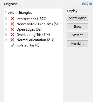
the following are the errors we need to clear before we set up the geometry. Before we set up, let's have a look at the geometry we have as.STL file.

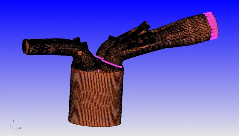
the colored marks the diagnose errors which we need to get rid of to achieve a clean setup for further case setup. We begin by running the diagnosis which we can do analyse the errors. We have the following errors:

Nonmanifolds Problems

Open edges

Overlapping Tris

Normal Orientations

Intersections

This is how we are going to clear all the errors and make the setup clean. First we are going to clear non manifolds error.

Non Manifold error

this is what that error looks like below

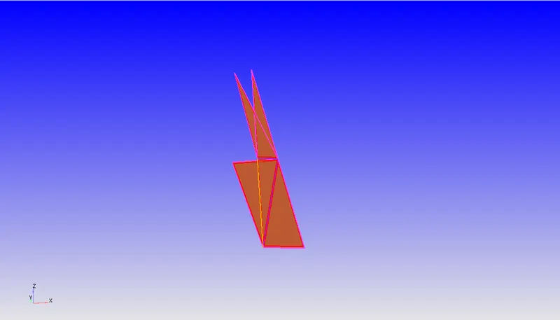
This error shows that there's an overlap of triangles is of quantity 5 so just deleting the overlapping triangles will clear the error. BY usi ng the tool DELETE under REPAIR section.

Open edges

The profile has some holes at the surface which are known as open edges. which is grouped by triangles and made edges free of connecting other triangles. Like this below:

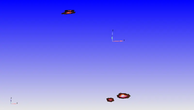
By Open Edge method we can PATCH it and the if necessary we can STITCH the unexpanded holes to fix the error.

Overlapping Tris and Normal orientations

These two errors are basically the same fixing any one of them will fix the others as you can see the location of both the errors below

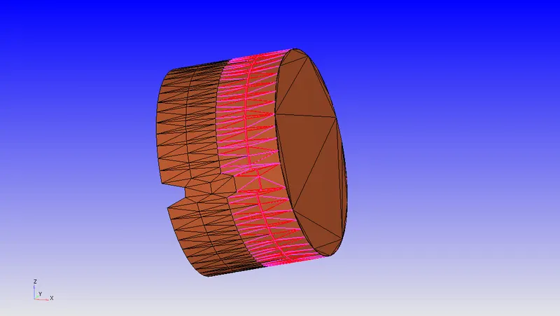
The Normal orientation is displaying NORMAL all over and reversing the normals on the inside of the geometry as the flows occur inside the geometry.

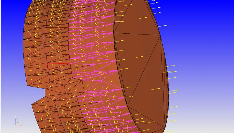
And reversing the NORMALS will fix both the errors.

Intersection:

This is a kinda error where triangles from the different boundary of the same or different regions may intersect that cause the flow to blow at the spots of the intersection. Before we dive into fixing the error, to make it simpler we assigned them boundaries to see what the major blow up at the profile.

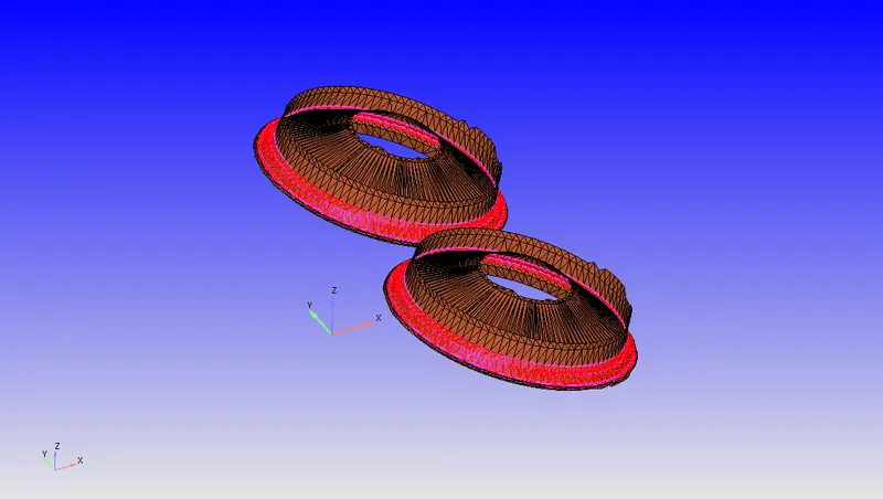
As you can see here the intersection of triangles at different boundaries in a nutshell. The different in colors helps identify the errors as below:

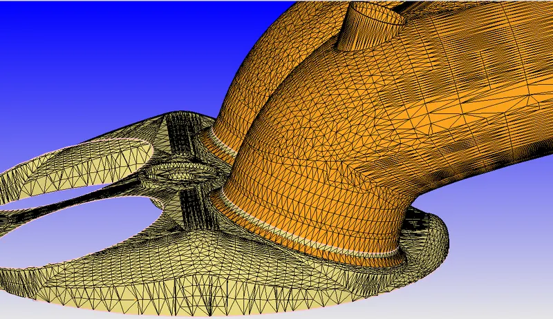
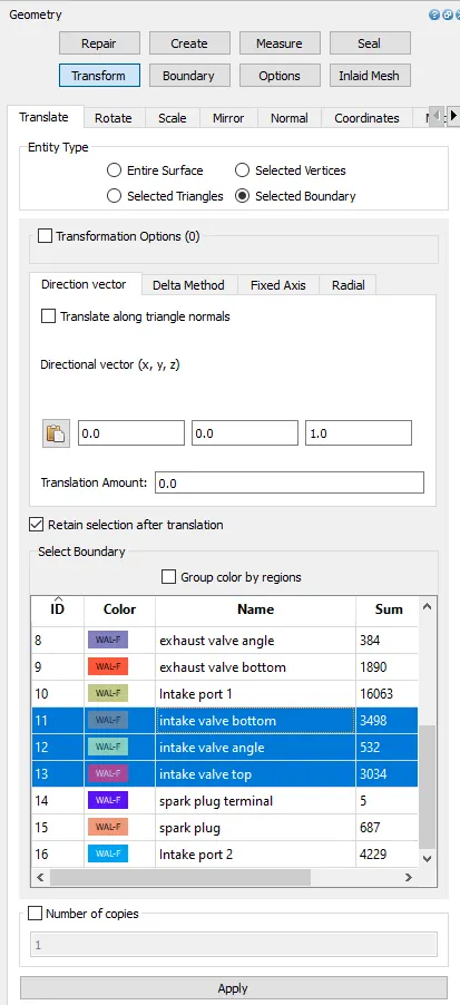
By using the translate tool we can always use the Transform tool for the selected boundaries to different angles or at different locations. Here in this case the Intake Port is made pushed into the cylinder head while designing the geometry in SOLIDWORKS or any other CAD package software. So what we are going to here is to Push back in little deep to make the section away from interesting point of interest. By using the Transform we can measure the ARC normals of the intake valve and for the selected boundaries we can Move them a little deep with a 0.001m translation amount with a directional vector inside the cylinder head.

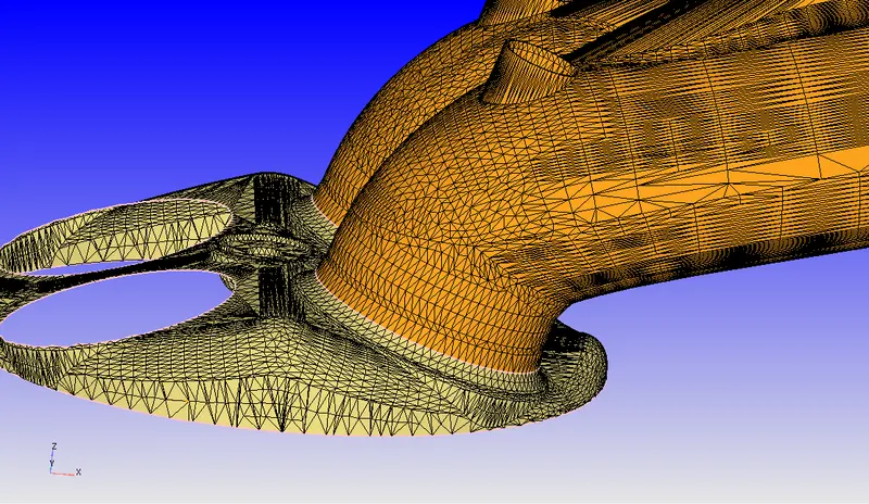
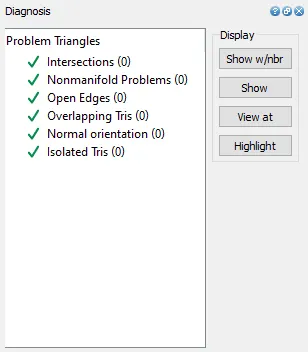
and we get very fined geometry with no errors at the end.

Now we are clear of the errors of the geometry we are going to start doing Boundary flagging at the earliest. Here after bouary flagging it should look like. These are the lists boundaries that should be flagged:

Piston

liner

Cylinder head

Intake port 1

Intake port 2

intake valve top

intake valve angle

intake bottom

Exhaust Port

exhaust valve top

exhaust valve angle

exhaust valve bottom

spark plug

spark plug terminal

inflow and Outflow.

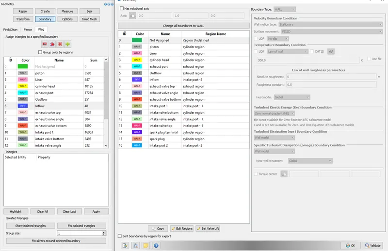
After boundary flagging, we are beginning to go for case setup for FULL HYDRO simulation, primarily we need to setup full hydro then after animation we can go for the FULL HYDRO. we can forward the case setup now. Now the Assigning all types of Technical parameters for the flow property to the case set up on the bottom right side. Below is the image is shown where all the case setup should like. The green tick indicates the all the parameter is set right according to flow properties. We can view this as below.

Assigning the boundaries is a must so that converge can recognize which is which to begin and understand the case setup part.

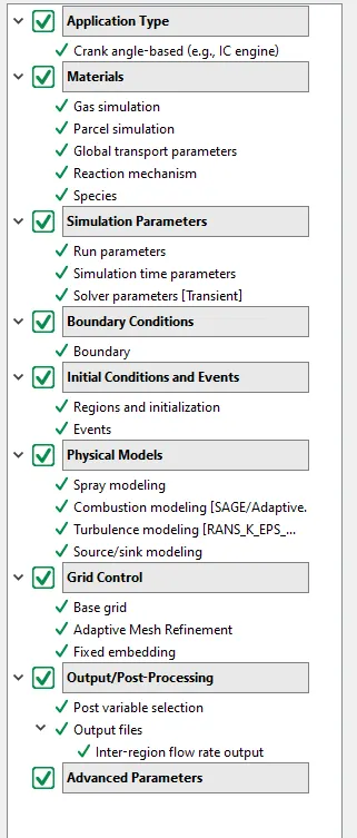
Before Jumping into the simulation part in Cygwin, one needs to set up the parameters in the case set up to look like the above image. The value represents in the above image shows the completion of the properties, here's how every section needs to be done.

Application type:

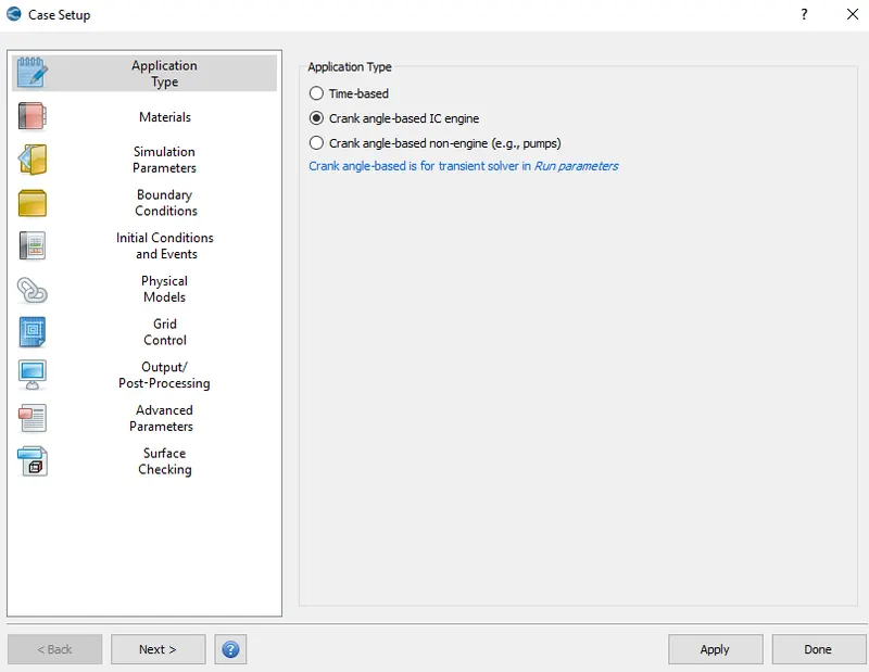
Selecting the Crank angle based IC engine is the option here as we are only setting up an IC engine based model simulation with a single stroke, to begin with, which is why we have to select this.

Materials:

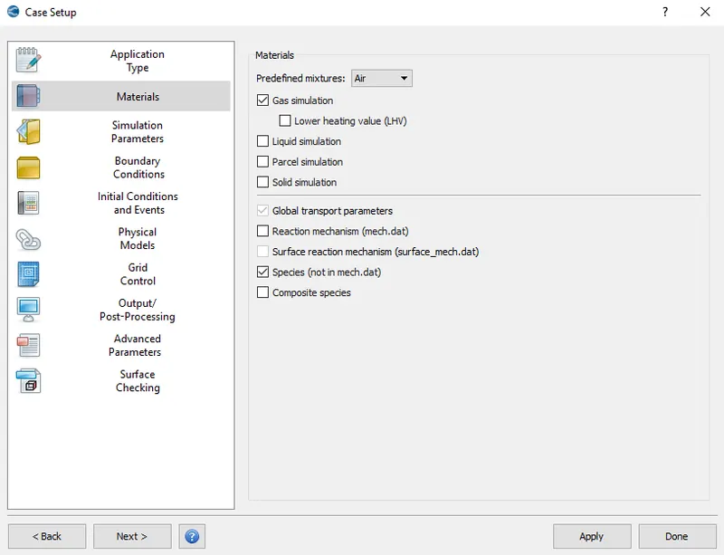
Here we have to assign some of the .IN files where we import all the data for the simulation. The mechanism here takes place as the result of combustion in the cylinder and Liner.

Gas Simulation:

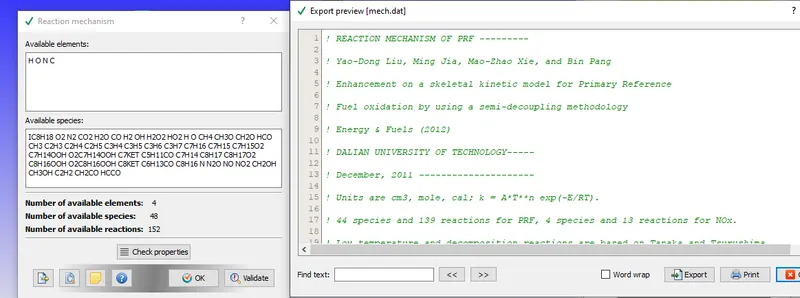
Here we import some of the data that are provided from an external source. so we are going to import therm.dat and mech.dat. this is how it looks while importing files.

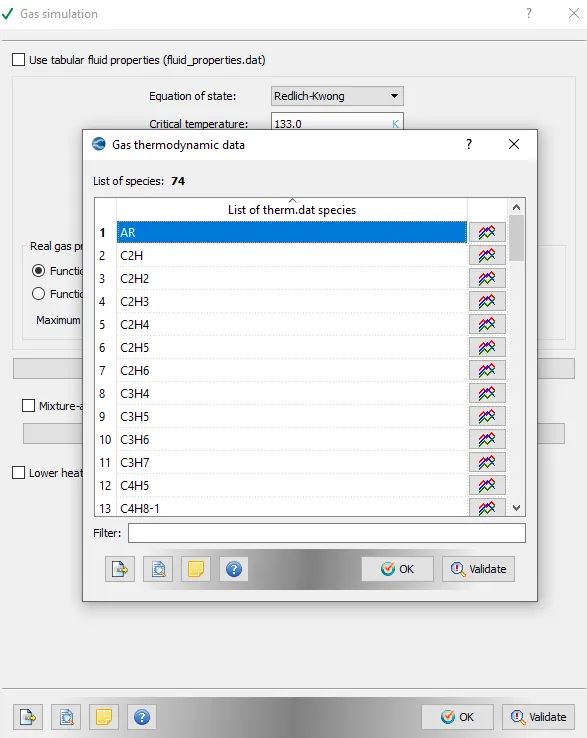
we don't do anything in the Global transport parameter a the input remains as it is.

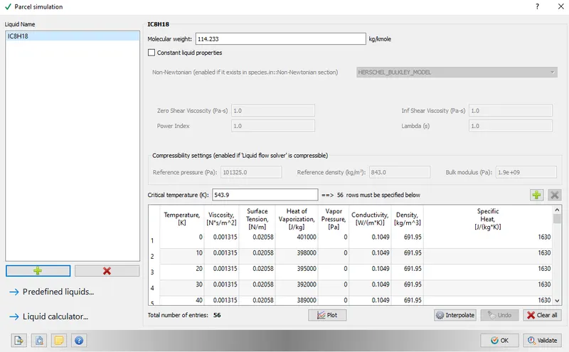
Parcel simulation: Here we have the details of Parcel paramtere for the simulation. what type of fluid showul be here for the parcel at the time of inflow we have taken here as iIC8H18 hydrocarbon for parcel simulations.

Reaction Mechanism:

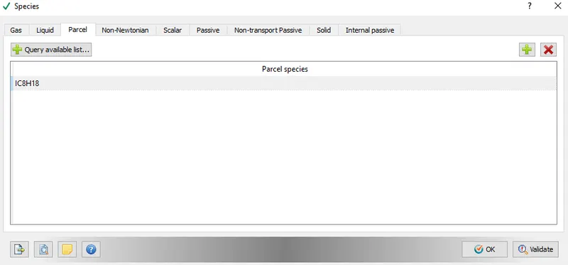
Species can be acquired in FULL HYDRO simulation that's what we gonna do heresince this is full hydro setup. we are going to ass PARCEL species as IC8H18

Moving on to Another section called Run Parameters where we assign very important terms to proceed.

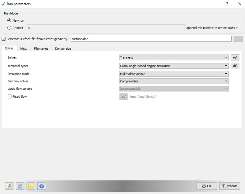
We select Transient solver in the solver section and Full hydrodynamics in the solver section because we are going for mesh generation on an IC-based engine. Where there is no complication in this system technically. The full hydrodynamic always take a lot of time to process the data files as it runs the basic Navier stokes equation through and through which might take a lot of time. Hydrodynamics would be a viable option when going for full hydro setup but again the fluid dynamics properties won't take place while running which is also quite an option in some cases.

Followed by Solver we have the Misc. option where we select the steady-state here again including unchecking the used memory option as we don't want extra storage for the simulation.

Assigning the value and validating it and Ok.

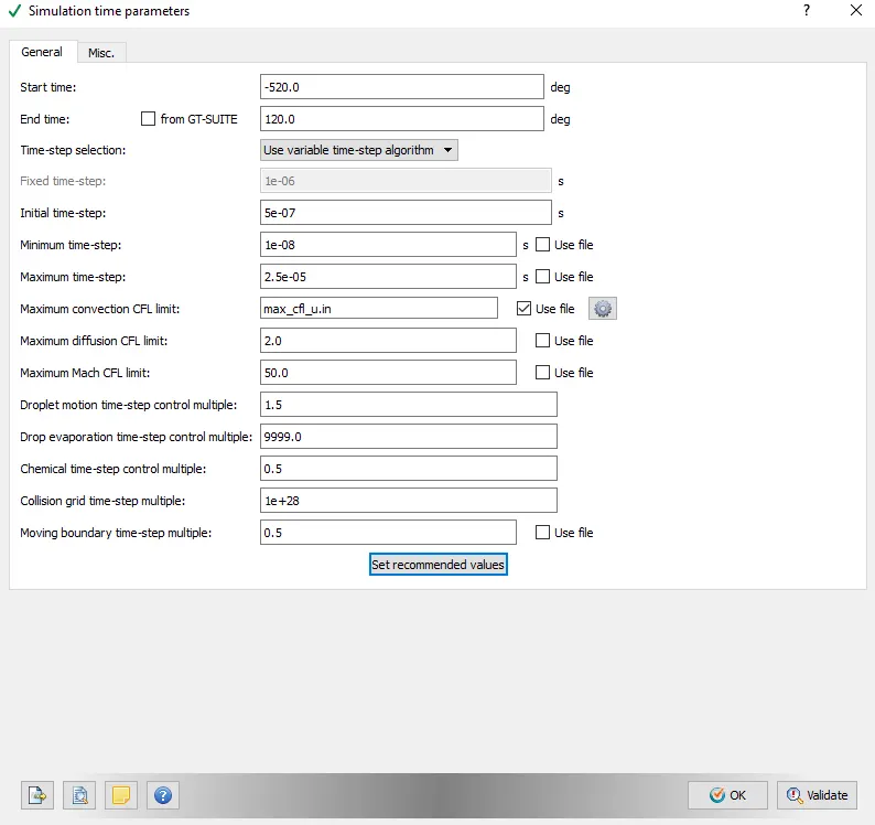
In another section called Simulation-Time Parametres here, we have all the values that are going to be involved in the simulation we are setting up.

The values here above for assigning. The start and end degree for the Cyclic nature of crank and valve motion will be -480 and 240

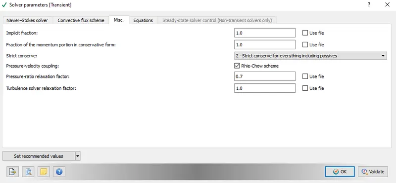
In the nest section of Solver-Parameters, we have what kind type of Navier-stokes solver, which is a Pressure-based solver for this flow.

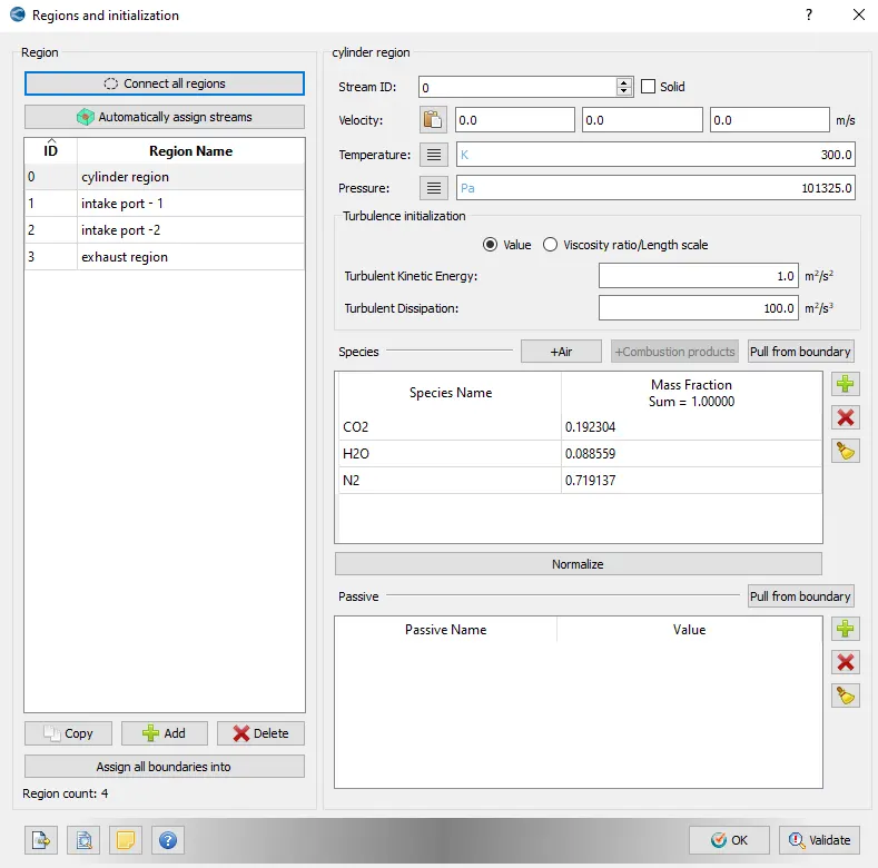
The next section is really important as we assign the Boundary condition for the flow and the walls around it to define the type of fluid flow effect on it while flowing. As we have done boundary flagging there we have established the boundaries in case setup. Hence here are going for the Region and Initialization.

Piston - Cylinder region

liner - Cylinder region

Cylinder head - Cylinder region

Intake port 1 - Intake port 1

Intake port 2 - Intake port 2

intake valve top - Intake port 1

intake valve angle - Intake port 1

intake bottom - Cylinder region

Exhaust Port - exhaust region

exhaust valve top - exhaust region

exhaust valve angle - exhaust region

exhaust valve bottom - Cylinder region

spark plug - Cylinder region

spark plug terminal - Cylinder region

inflow - Intake port 2 and Outflow - exhaust region

For all the exhaust region awe have Exhaus_lift.in file which get imported and same goes for Intake_lift.in

here we have only as much boundaries as there are above mentioned. for assigning the whole region we have to create region with appropriate inputs that need to be considered.

In the Region and Initialization, We need to add the cylinder region, intake port 1, intake port 2 and exhaust region and calculate the stoichiometric of h20 n2 and co2 and we get the following values are as below. for cylinder region, exhaust region and we import the boundaries from OUTFLOW.

Now here was have an interesting tool that describes the flow motion of fluid from regions to regions. Its called the EVENTS. we need to put values right like as:

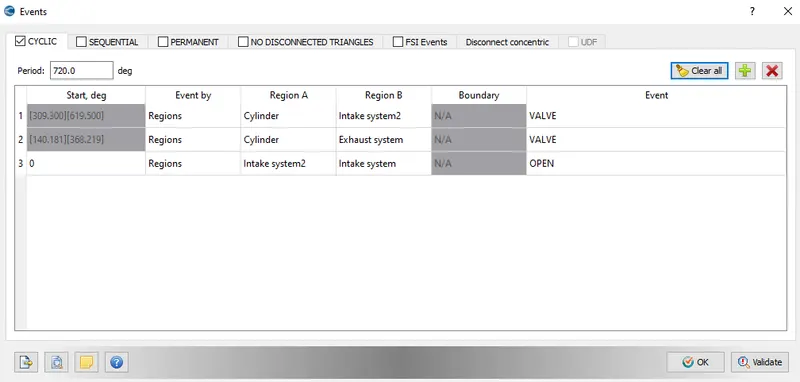
here we commanding the software to CLOSE the regions at 0 and OPEN at 0.001 so the fluid flow can take place from high to low and it gets good motion flowwith regions A and Regions B.

IN the Physical-Modelling We need to check the turbulence modeling as there will be turbulent flow over a channel because of the throttle body. We select the RNG k e method to solve the analysis.

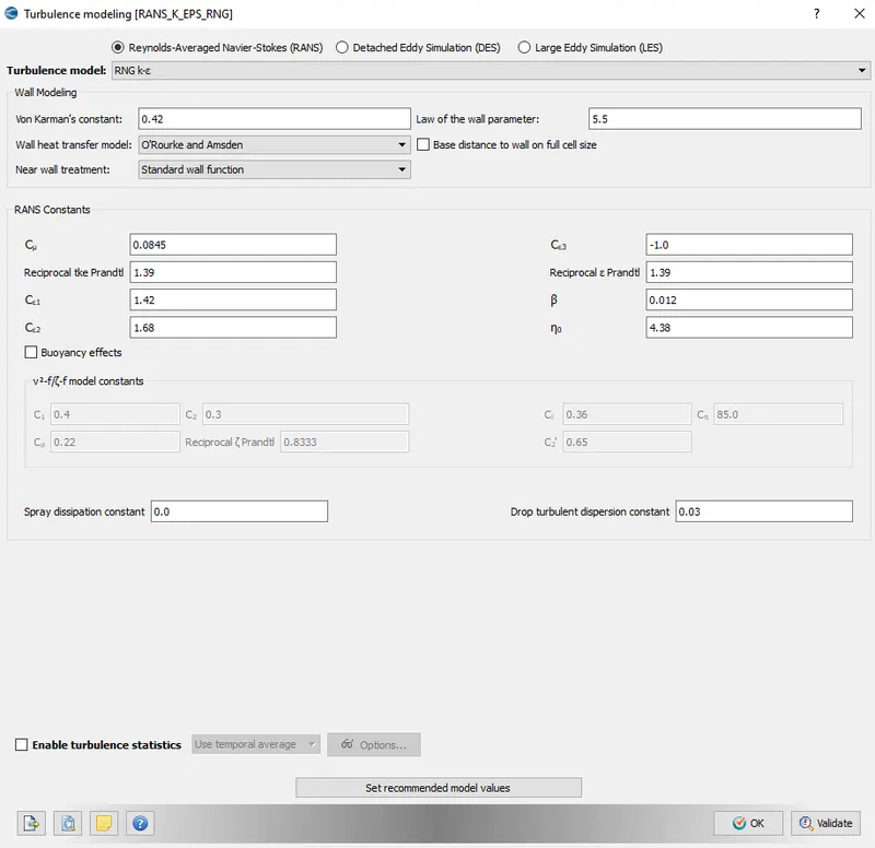
another option we here is the Spray modelling. The spray pattern should be feasible for parcel generation into the system. the details are below.

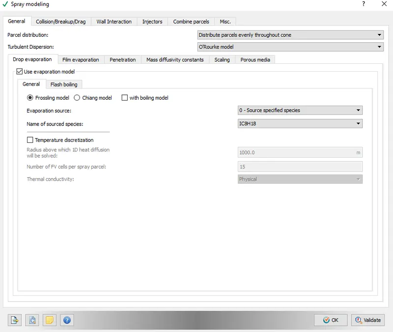
another modeling we ned to focus on is the Combustion modelling. Since we are doing the full hydro simulation we need to bring combustion setup happening inside the IC engine into the consideration. The modelling sets the compxcity of the simulation.

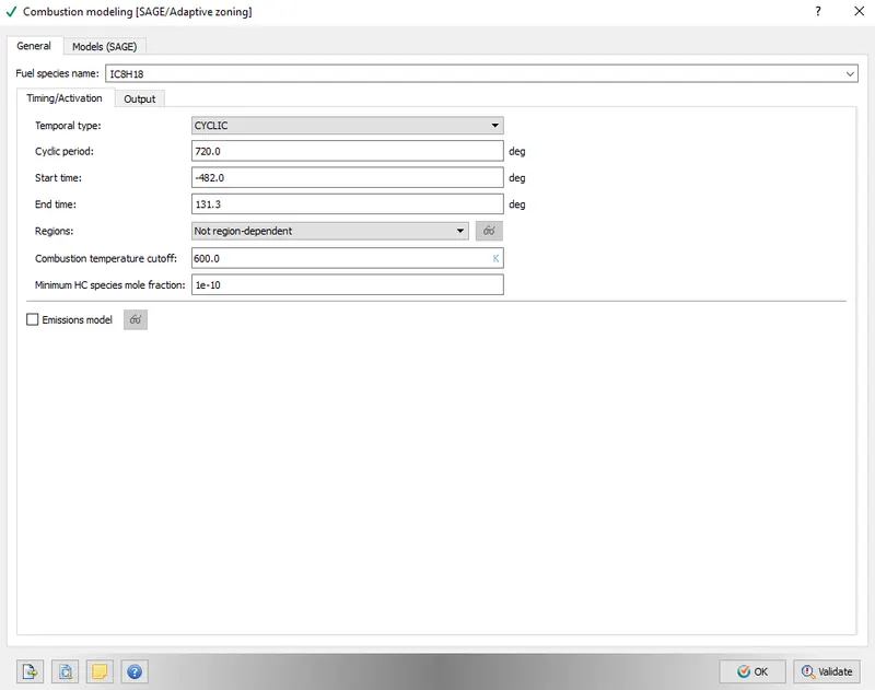
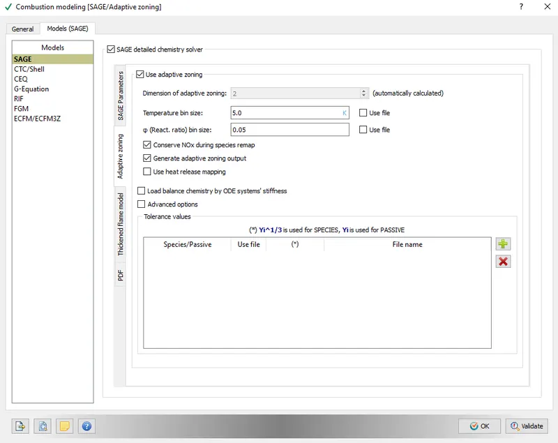
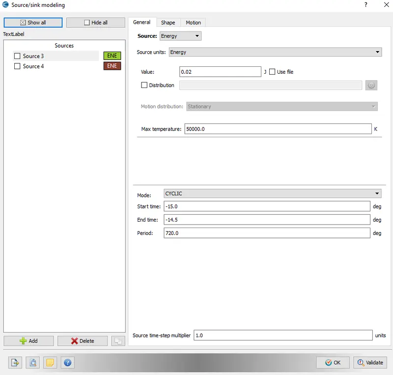
Next we have is Source/sink modelling

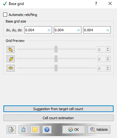
Now the next section is Base Grid, where we assign the INPUT coordinated for the channel so that it has a different output for different inputs. This where the box we create in the first stem gets its own assigned values of coordinates in a cartesian plane.

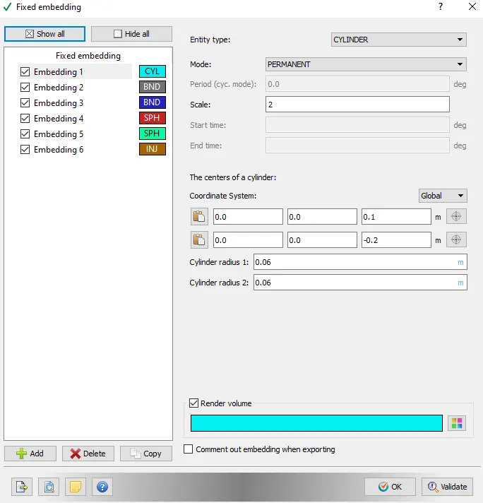
And again we have here Fixed Embedding where we are going to give some values so at the shock flow the refinement takes place with mesh looks more clear. But we are not going include it as it crashes the simulation inlower configuration system with 4 cores. we need supercomputer to get it running.

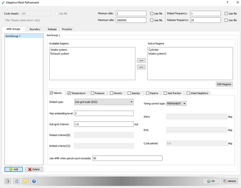
Adaptive Mesh refinement

again we have here POST VARIABLE SELECTION we are just going to leave as it is. As we are not doing the full hydro.

With the SIMULATION oof OUTPUT FILES we have here:

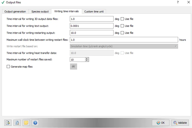
And now we are finally done with setup case and moving onto simulation followed by POST PROCESSING 3D files.

But before we move on to post processing the data files we have some theoretical research based questions that we need to understand and determine.

1. What is the compression ratio of this engine?

The compression ratio is defined as the ratio between the volume of the cylinder with the piston in the bottom position, V_bottom (largest volume), and in the top position, V_top (smallest volume). The higher this ratio, the greater will be the power output from a given engine. It is generally in the 6-10 range.

	=	static compression ratio
	=	displacement volume
	=	clearance volume

in our case the Vmax is 0.000961785 and V min is 0.000439572 from the plot we have on the Converge we are safe to say the our Compression Ratio is 1.0058

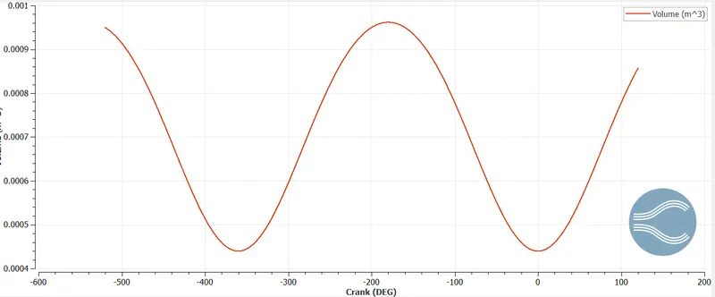
as we can see here the Vmax and Vmin here.

2. Why do we need a wall heat transfer model? Why can't we predict the wall temperature from the CFD simulation?

Internal combustion engines are now extremely optimized, in such ways improving their performance is a costly task. Traditional engine improvement by experimental means is aided by engine thermodynamic models, reducing experimental and total project costs. For those models, accuracy is mandatory in order to offer a good prediction of engine performance. Modeling of the heat transfer and wall temperature is an important task concerning the accuracy and the predictions of any engine thermodynamic model, although it is many times an overcome task. In order to perform a good prediction of engine heat transfer and wall temperature, models are required to accomplishing heat transfer from hot gases to engine parts, heat transfer inside each engine part, and also heat transfer to coolant and lubricating oil.

The most important correlation is reviewed for three engine heat transfer approaches gas to the wall, wall to wall, and wall to liquid heat transfer models. In order to obtain a good prediction of wall temperature, those three approaches must be coupled, which may imply convection-conduction-convection problems, although, for some applications in diesel engines, radiation problems must be considered.

Direct CFD simulation of conjugate heat transfer problem or Wall temperature can be too difficult in the case of multi-layered structures with internal cavities. But there are other possibilities. For example, Star-CD offers such an option as specified heat flux through the wall. This allows us to run the simulation with a simple “hole-in-the-mesh” approach, calculating the heat flux through the wall with some simple tool and correcting the boundary value, say, every 100 computational steps. Such an approach yields only a slight increase in computational expenses and gives much more accurate results than using adiabatic wall conditions. But these accurate results also have cons for the computational period.

3. Calculate the combustion efficiency of this engine

Combustion efficiency is the calculation/measurement, in percentage, of how well your equipment is burning a specific fuel. Complete combustion efficiency (100%) would extract all the energy available in the fuel. However, 100% combustion efficiency is not realistically achievable. Various combustion processes produce combustion efficiencies from 0% to 95⁺%. Combustion efficiency calculations assume complete fuel combustion and are based on three factors:

1. The chemistry of the fuel.
2. The net temperature of the stack gases
3. The percentage of oxygen or CO₂ by volume after combustion.

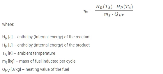
but we have here as Combustion Efficiency = Heat release/ Total Energy content.

from the IHR graph, we can determine the Heat Release

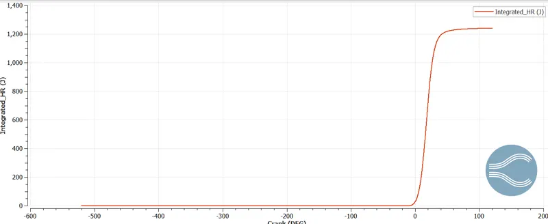
Heat release = 1242J

Total Energy Content = Cv x mf

where Cv here is calorific value

Cv of Gasoline is 44Mj/kg

Fuel Mass of percycle = 3 x 10^-5 kg

Total Energy = 44 x (3x10^-5)J = 1320J

Combustion Efficiency eta = (1242/1320)x 100 = 94%

4. use the engine performance calculator, to determine the power and torque for this engine. Since Work and Torque have the same unit (N-m), it doesn't mean the value for Torque and Work will be the same. Both are different quantities and has totally different meaning. So the value for work that you will be getting from the engine performance calculator is not the value for the torque. Calculate the value for the torque using the formula as shown below?

Power(P) = (2*π*N*T)/60

For work done we need to calculate from an engine calculator tool in COnverge. In here we have to select thermo.out file and engine.dat file for the inputs needed.

Rpm = 3000

RPS = 3000/60

DPS = RPS.360 = 18000

time 720 degree = 1/18000 * 720 = 5.5 e-5.240 = 0.0133 time taken for one cycle of operation

P = Work Done/ Time taken = 468.64/0.0133 = 35.5

T = Px60/2x3.14xN = 111.9 Nm

5. What is the significance of ca10, ca50, and ca90?

The physical significance of CA10 is that it is used to identify the start of ignition in a diesel engine, whereas the CA50 indicates the end of premixed combustion and the start of diffusion combustion of fuel used in the engine. The higher the difference between CA10 and CA50 (CA50-CA10), the higher will be the combustion duration and vice versa. In the present study, the CA50-CA10 is observed to be higher for the PD mode in contrast to the DFD mode of engine operation. same goes for ca 90.

Output:

Animation of Port Fuel Ignition IC engine.

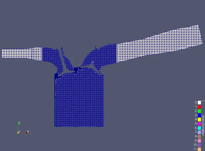
Mesh Generation at surface with edges

Plots:

Pressure:

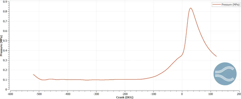
pressure in the cylinder varies with the varying crank angle at different stokes. the pressure is high at the end of the compression stroke and decreases when expansion takes place. The peak pressure reaches here is 0.85Mpa.

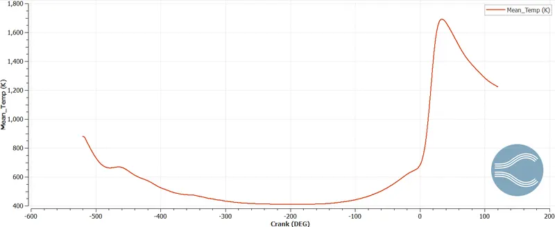
Temperature

Volume:

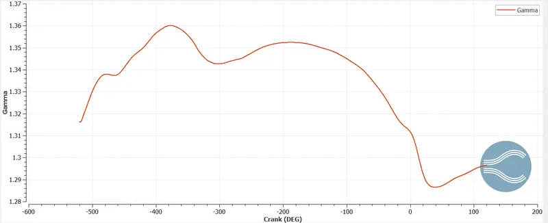
Gamma value:

Integrated Heat release is total energy releasing in the combustion process.

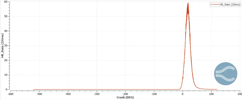
Heat Release Rated

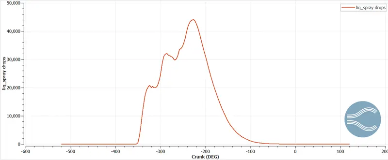
Liquid Spray

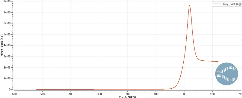
EMISSIONS :

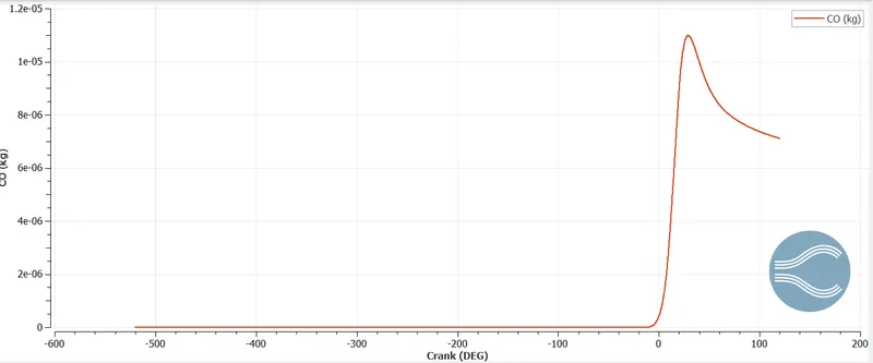
Some emission hydrocarbons are here NOx, hiroy soot, and carbon monoxide.

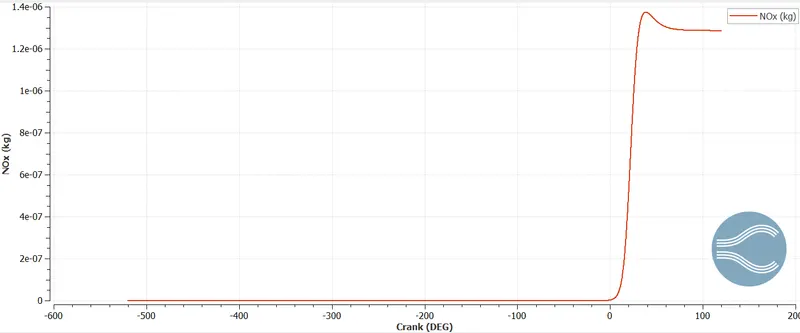
Nitrogen gets produced in a combustion reaction phase which is toxic in nature. The maximum NOx produced here is9e-7 kg and the reduced to 8.6e-7 kg.

Conclusion:

The Full hydrodynamics PFU setup ran successfully with accurate values in a combustion process.

here we have taken Spray modeling, Turbulence modeling, Mesh refining techniques, and parcel simulation and reaction mechanism into account t which made us determine the volumetric parameters of the data in the combustion process.

Adaptive mesh refinement and fixed embedding features are performed to make mesh look refined.