Aim:

To simulate SI8 PFI engine Full hydro case setup using Converge Studio and to post process the results.

Given Conditions and parameters :

Engine Geometric Parameters

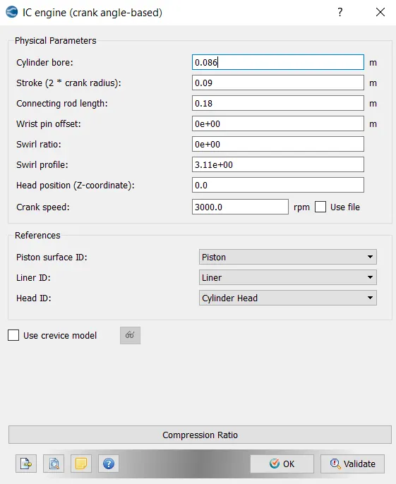
1. Bore =0.086 m
2. Stroke = 0.09 m
3. Connecting rod length = 0.18 m
4. RPM = 3000

Run parameters

1. Simulation mode: No Hydro

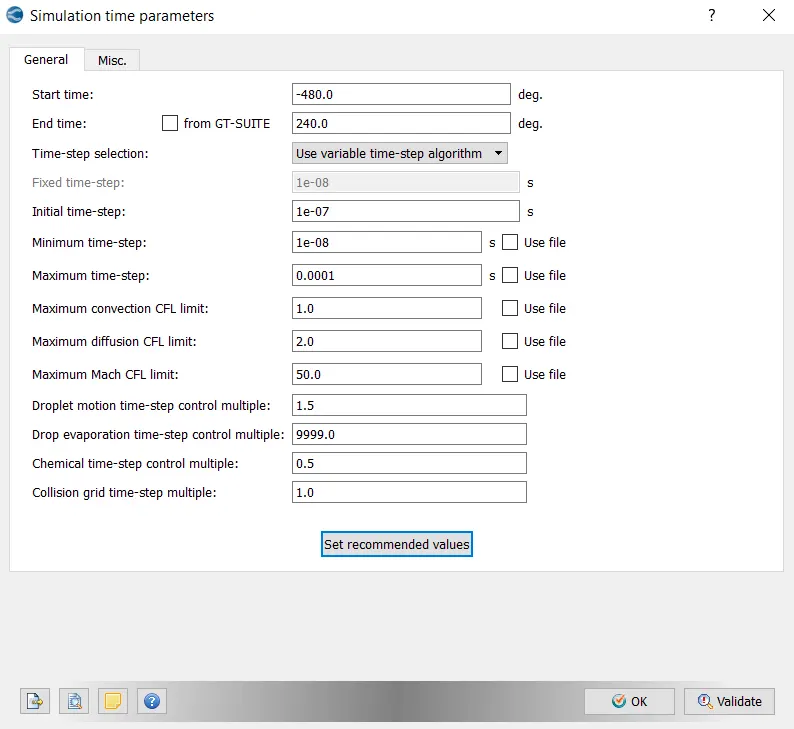
Simulation time parameters

1. Start time : -520 deg
2. end time : 120 deg

Boundary conditions

1. Piston temperature - 450K
2. Liner temperature - 450K
3. Head temperature - 450K
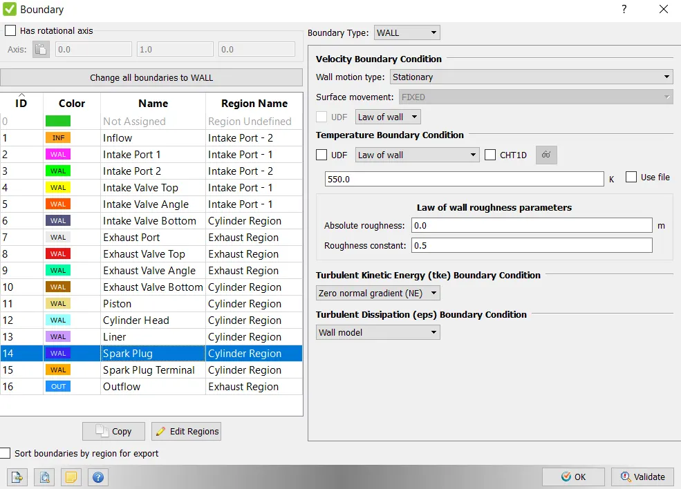
4. Spark Plug temperature - 550K
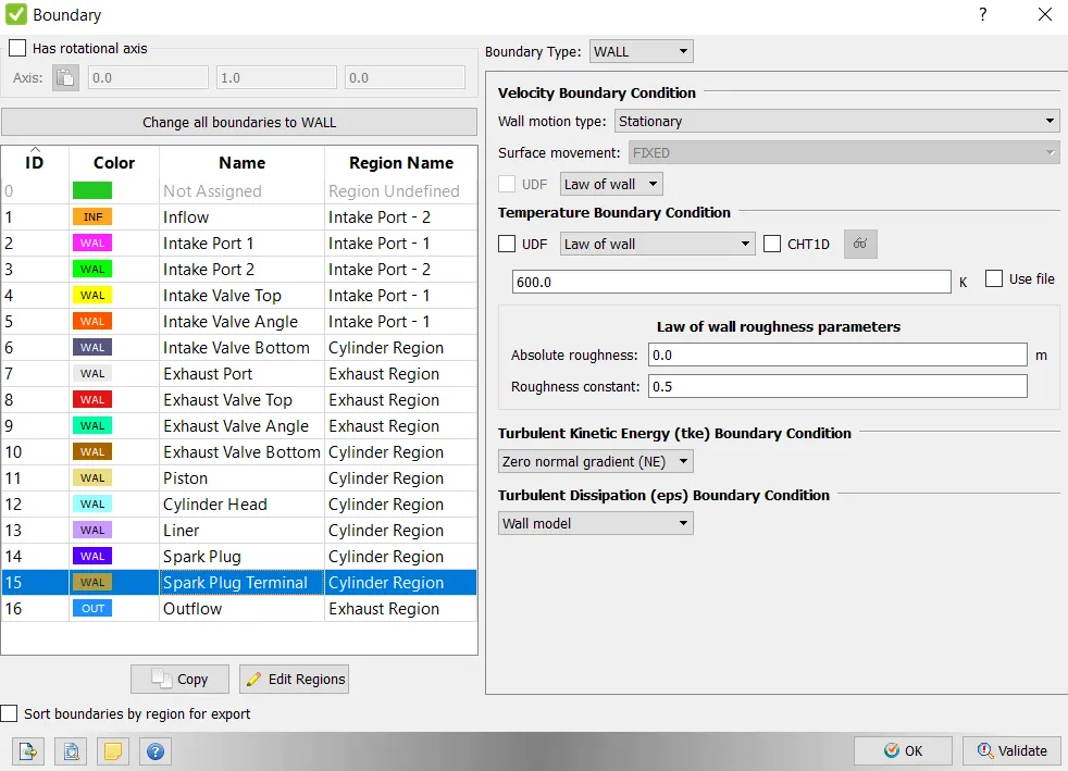
5. Spark Plug electrode temperature - 600K
6. Exhaust ports temperature - 500K
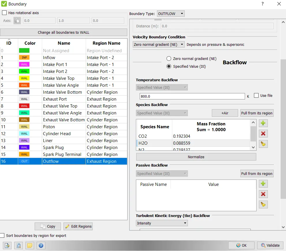
7. Exhaut outflow - 1 bar
8. Exhaust outlflow temperature - 800k
9. Exhaust species concentration - Calculate the stoichiometric condition
10. Exhaust valve top temperature - 525K
11. Exhaust valve angle temperature - 525K
12. Exhaust valve bottom temeprature - 525K
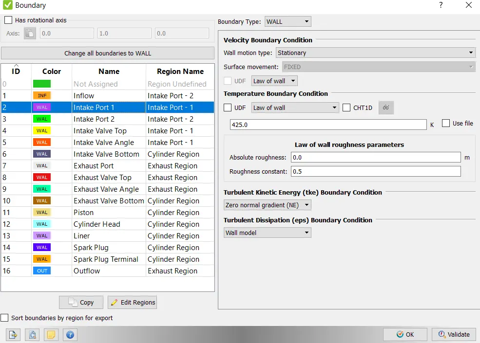
13. Intake port - 1 temperature 425K
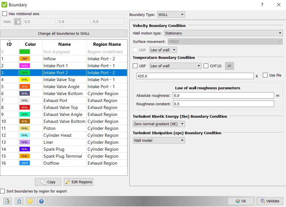
14. Intake port - 2 temperature 425K
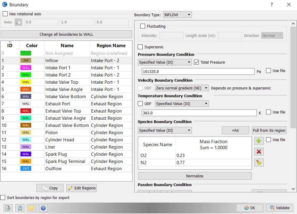
15. Inflow pressure - 1 bar total pressure
16. Inflow temperature - 363K
17. Inflow species - Air
18. Intake valve top temperature - 480K
19. Intake valve angle temperature - 480K
20. Intake valve bottom temeprature - 480K

Initial conditions

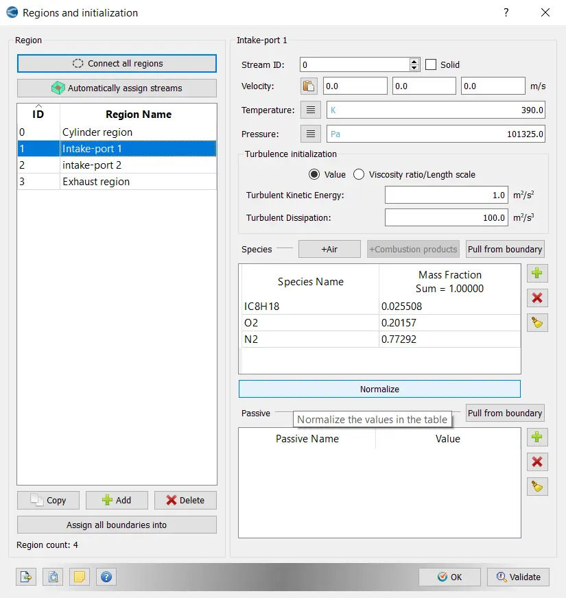
• Intake port - 1 (closer to combustion chamber)
  • ic8h18 - 0.025508
  • o2 - 0.20157
  • n2 - 0.77292
  • Temperature - 390k
  • pressure - 1 bar
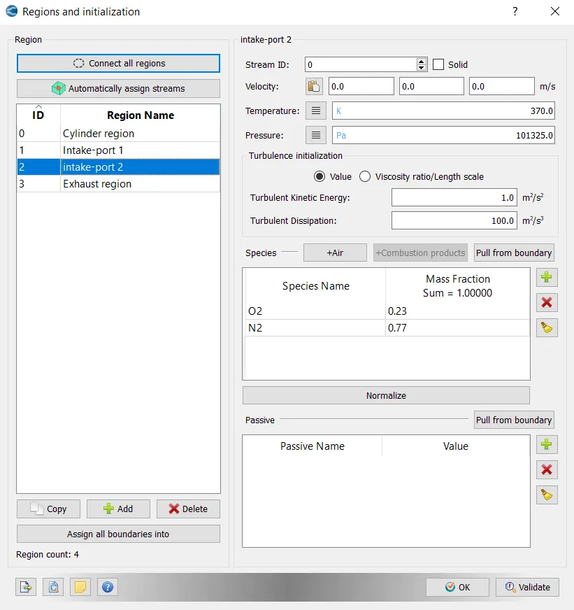
• Intake port - 2 (away from combustion chamber)
  • Air
  • Temperature - 370K
  • Pressure - 1 bar
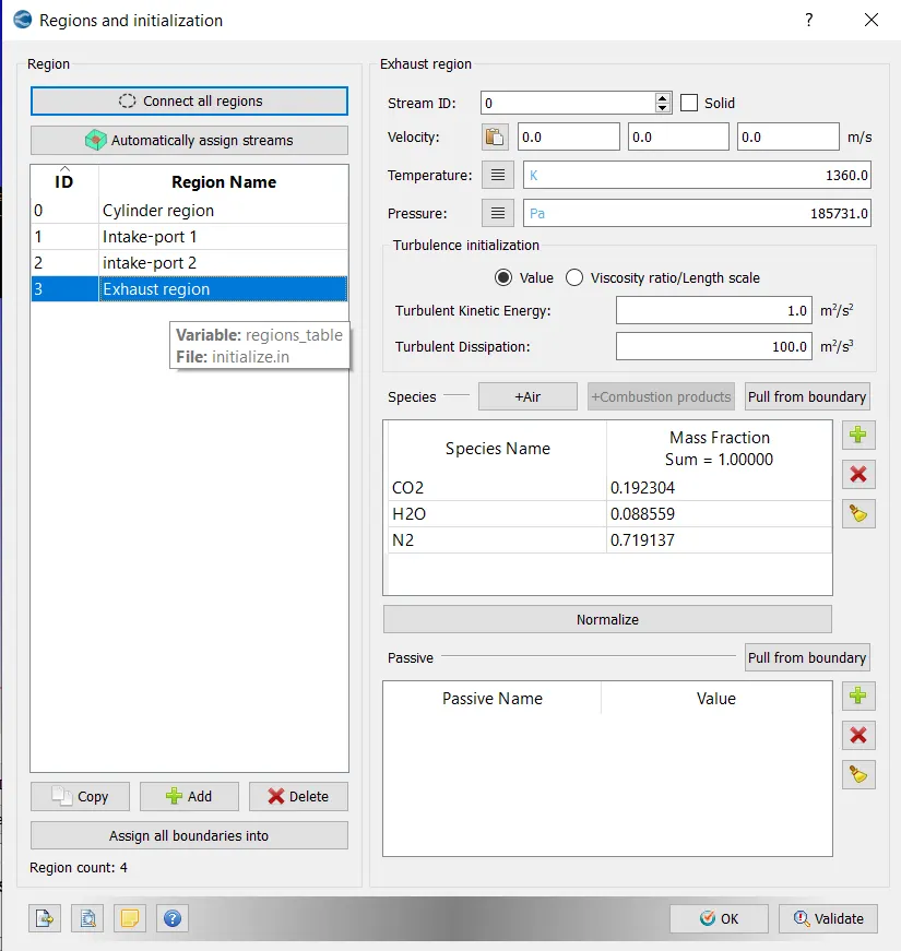
• Cylinder
  • Pressure - 1.85731 bar
  • Temperature - 1360K
  • Stoichiometric composition

Injection Parameters

1. Fuel flow rate = 7.5e-4 Kg/second
2. Injection start time = -480.0
3. Injection duration = 191.2
4. Fuel temperature = 330K

Nozzle positions

Nozzle diameter = 250 micro-meter

Circular injection radius = Nozzle radius

Spray cone angle = 10

• Nozzle 0
  • center 0.0823357 0.00100001 0.07019
  • Align Vector -0.732501 0.210489 -0.647408
• Nozzle 1
  • center 0.0823357 -0.00099999 0.07019
  • Align Vector -0.732501 -0.210489 -0.647408
• Nozzle 2
  • center 0.0823357 -0.0004 0.07019
  • Align Vector -0.5 -0.2 -0.647408
• Nozzle 3
  • center 0.0823357 0.0003 0.07019
  • Align Vector -0.5 0.2 -0.647408

Spark Ignition Parameters

• Start of spark = -15 deg
• Spark duration = 10 deg
• Spark location = -0.003 0 0.0091
• Spark radius = 0.0005m

Objectives:

1.What is the compression ratio of this engine?

2. Why do we need a wall heat transfer model? Why can't we predict the wall temperature from the CFD simulation?

3. Calculate the combustion efficiency of this engine

4. use the engine performance calculator, to determine the power and torque for this engine.

So the value for work that you will be getting from the engine performance calculator is not the value for the torque.

Calculate the value for the torque using the formula as shown below,

Power(P) = (2*π*N*T)/60

5. What is the significance of ca10, ca50 and ca90?

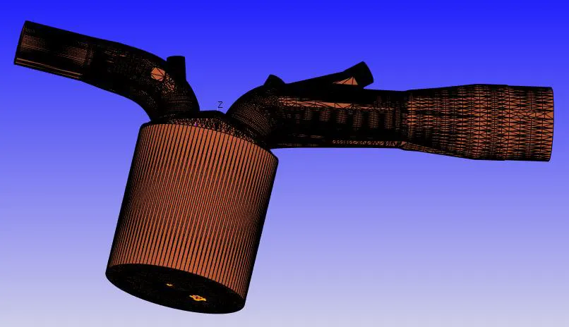
Given Geomentry:

Diagnosis:

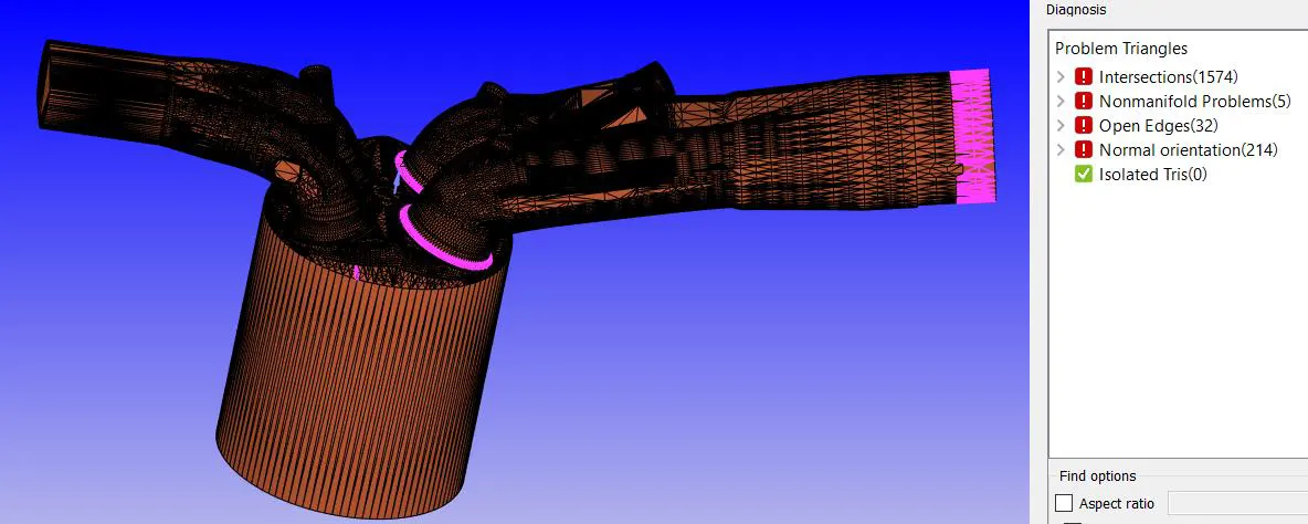
Intersection Error:

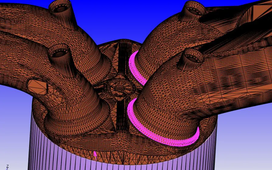
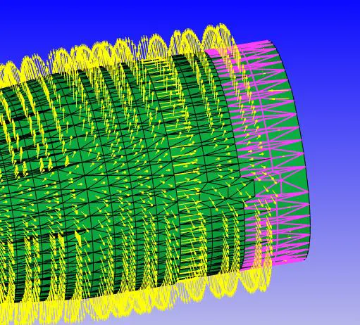
While flagging cylinder head, we can find that there are intersection errors (indicated in pink). This is because the valves of inlet side are superimposed on the head as it was lifted high. We need to translate it to the position where these intersection errors are eliminated

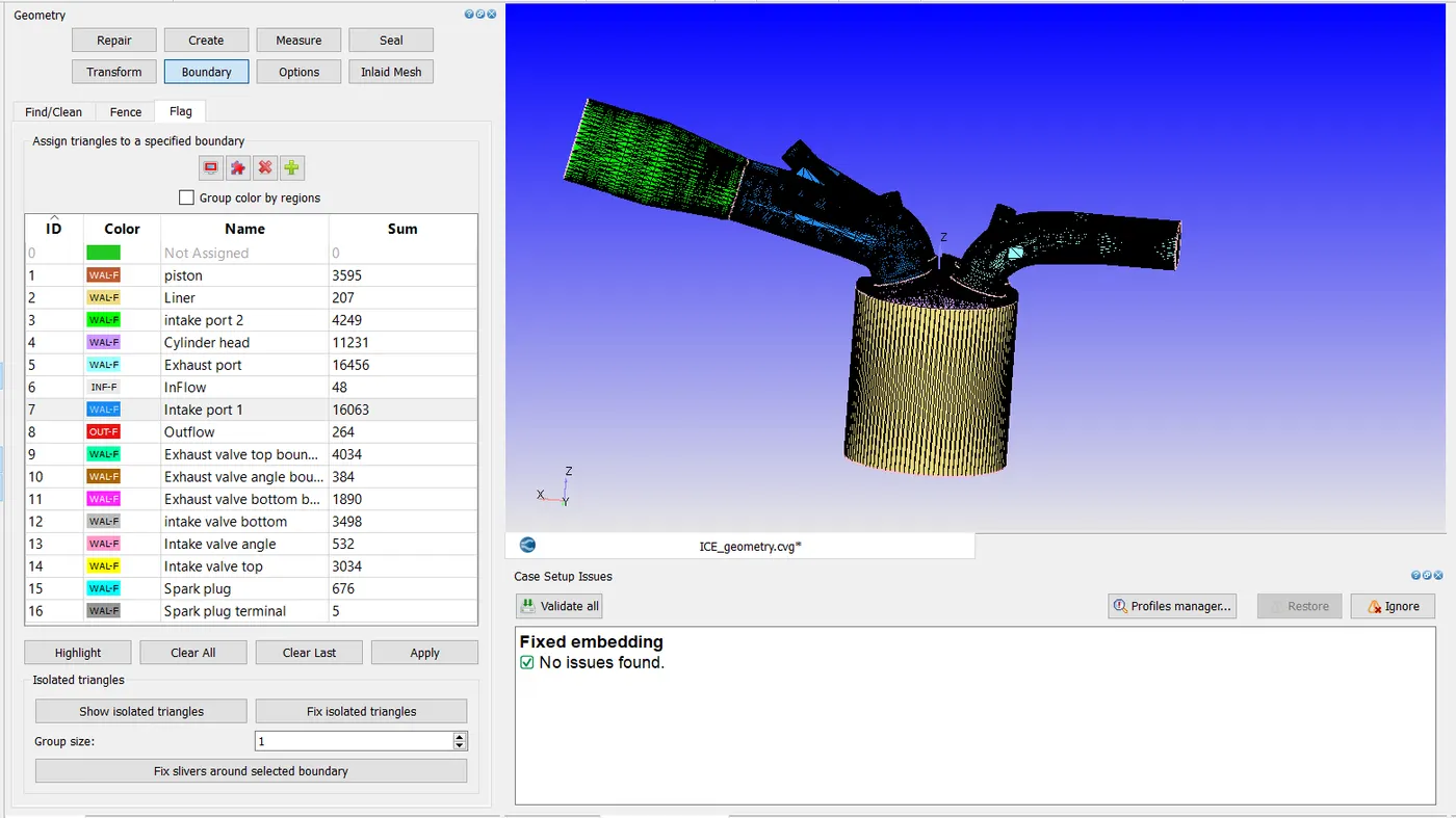
Surface preparation and boundary flagging:

Inflow Boundary

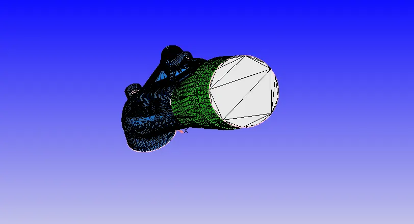
Outflow Boundary

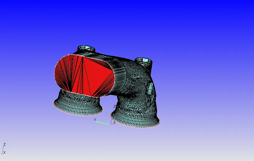
Piston

Liner

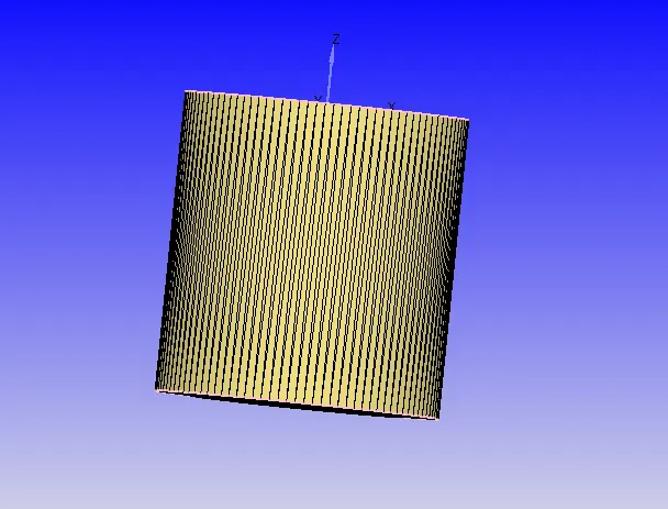
Intake and Exhaust Valves

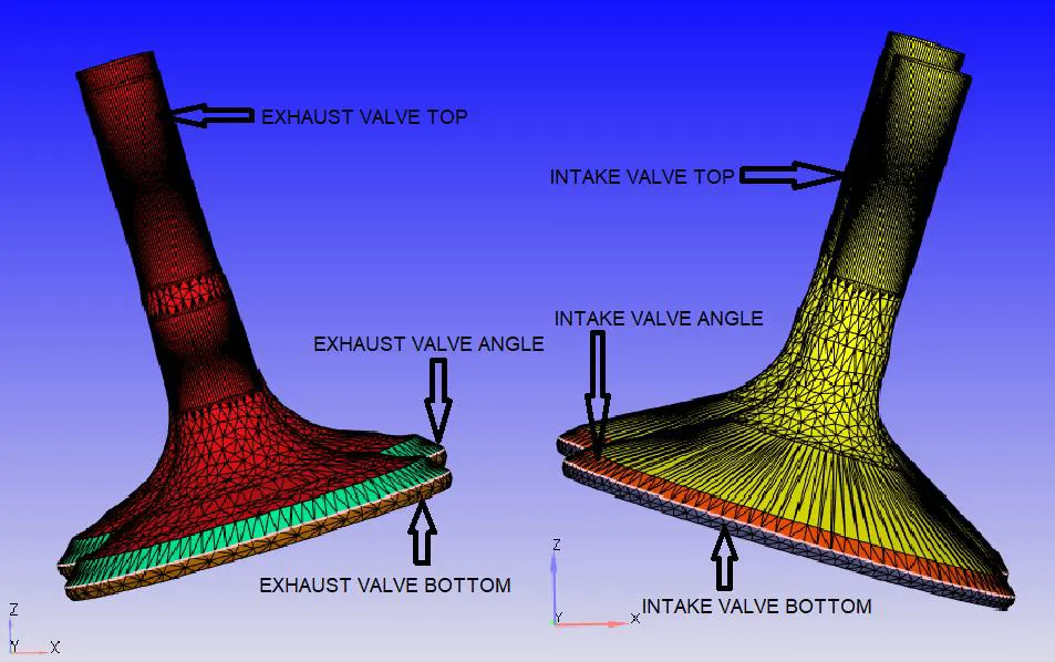
First, the intake and exhaust valves are divided into three sections namely top, angle and bottom and are flagged accordingly. Then the intake valve is translated down to eliminate intersection errors with cylinder head.

Exhaust Port

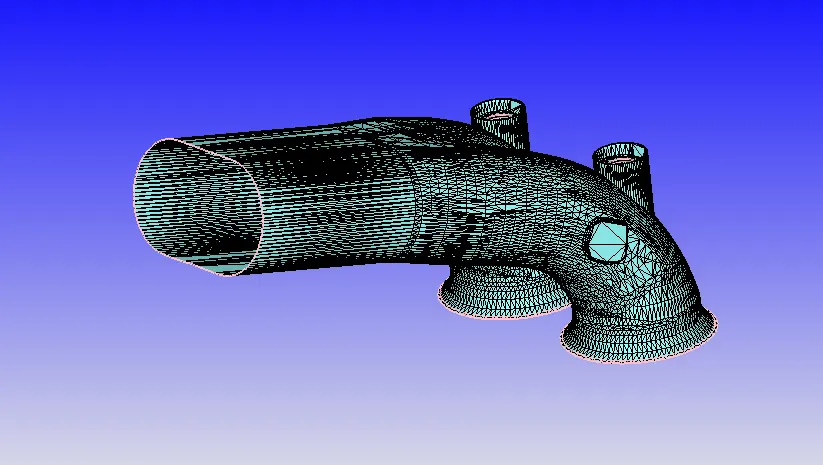
Intake port

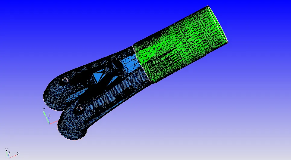
Sark Plug and its terminal

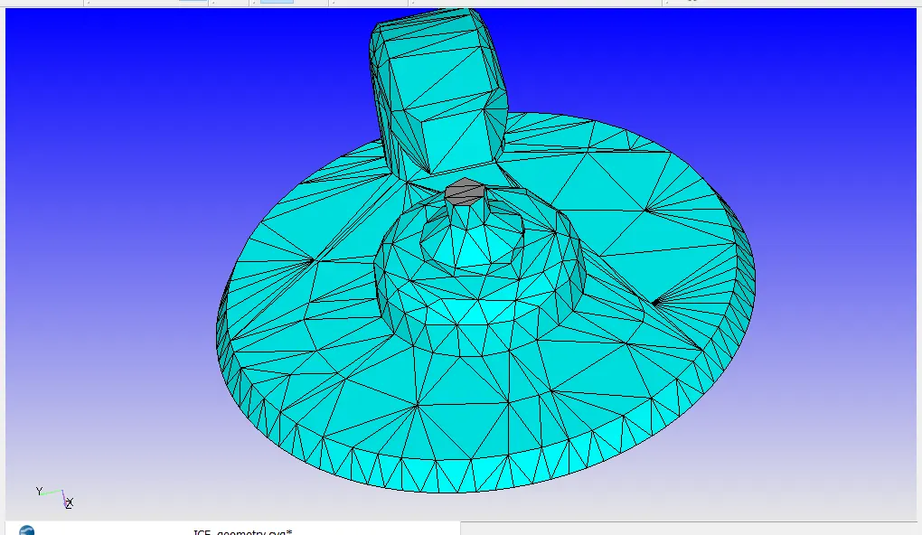
Ring triangles translated

To remove the superimposing errors, we need to create boundary fences and extend the port boundaries close to the valve boundaries. Make the three point arc on the circumference of the circle (Ring triangles – used to avoid deformation in valve geometries during translation). This co-ordinates are taken and translated or pushed down by 1mm to remove the intersection errors.

Cylinder head

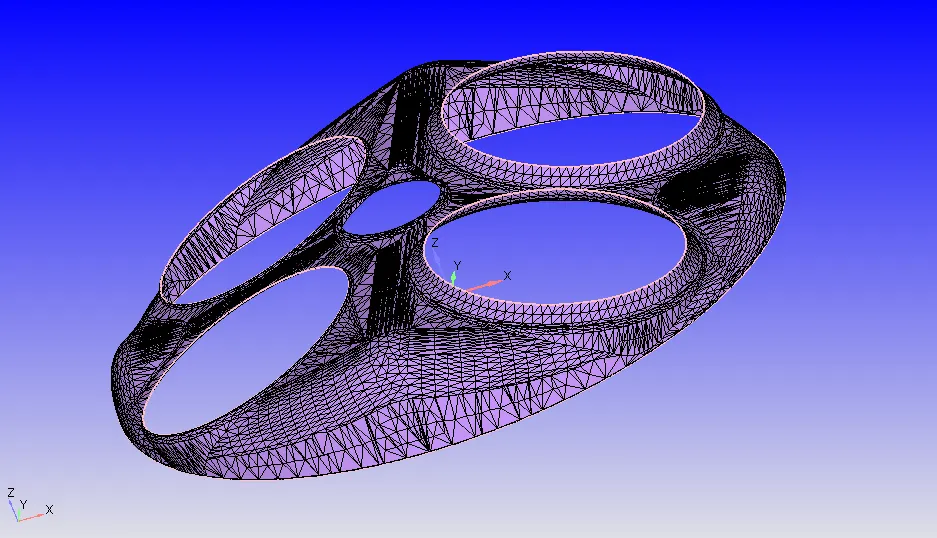
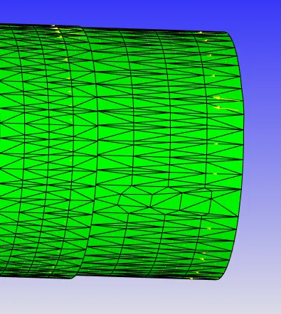
Normal pointing

Completed Boundary flagging and regions:

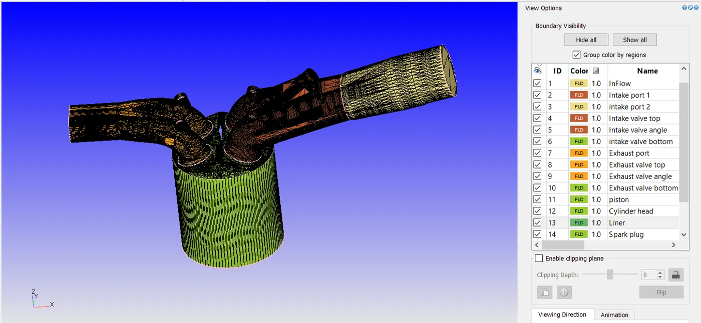
Four regions are created:

Cylinder region:

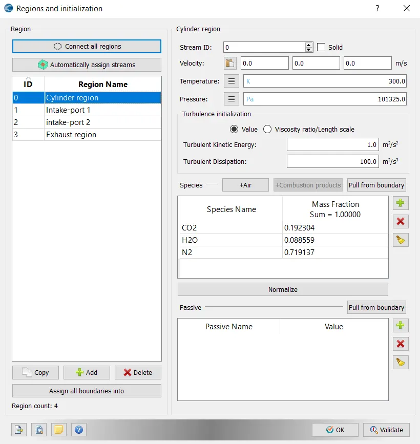
Intake part 1:

Intake part 2:

exhaust region:

CASE SETUP FOR Full HYDRO SIMULATION:

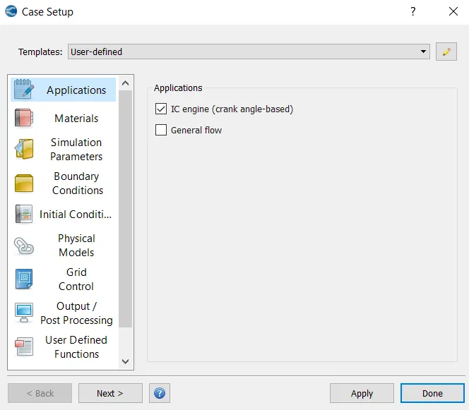
IC Engine Application

Parameters of PFI Engine

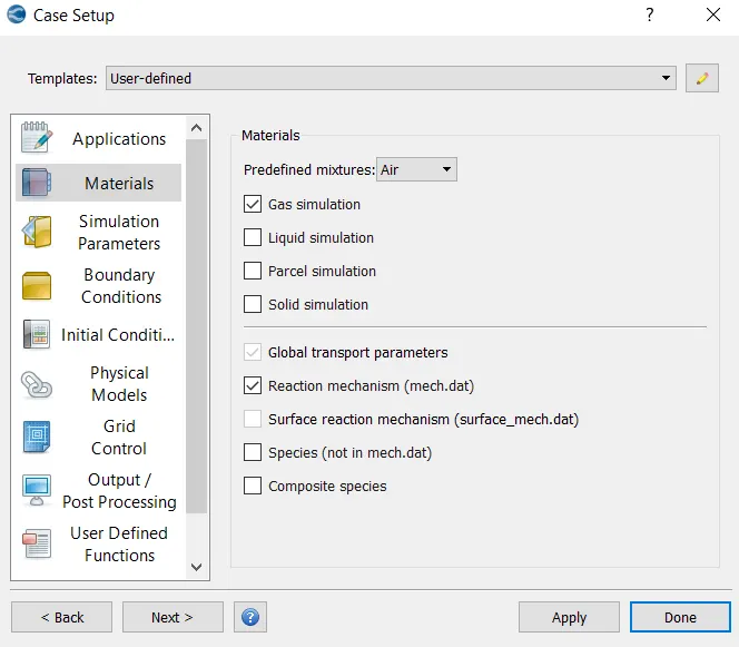
Materials

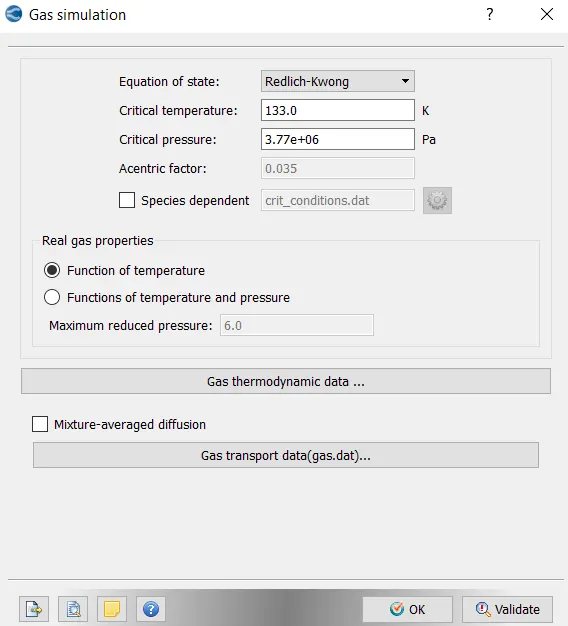
Gas Simulation

PARCEL SIMULATION

Enabling Parcel Simulation

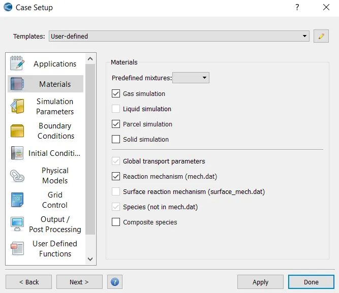
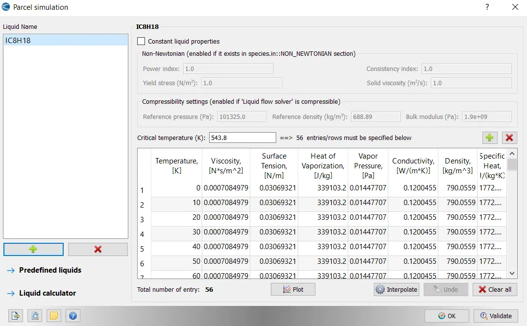
In the parcel simulation, the predefined liquids option is clicked and the fuel IC8H18 is selected from the list of available liquids.

Specifying species:

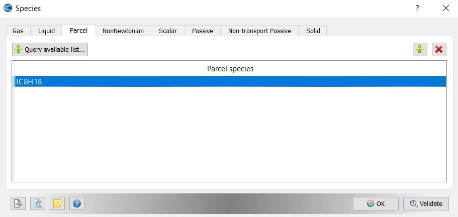
Gas species is taken care in reaction mechanism itself. Select parcel species as IC8H18

Global Transport Parameters

Reaction Mechanism

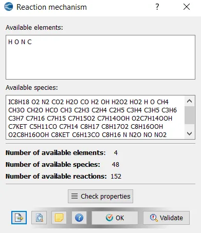
(Imported from the given mech.dat file)

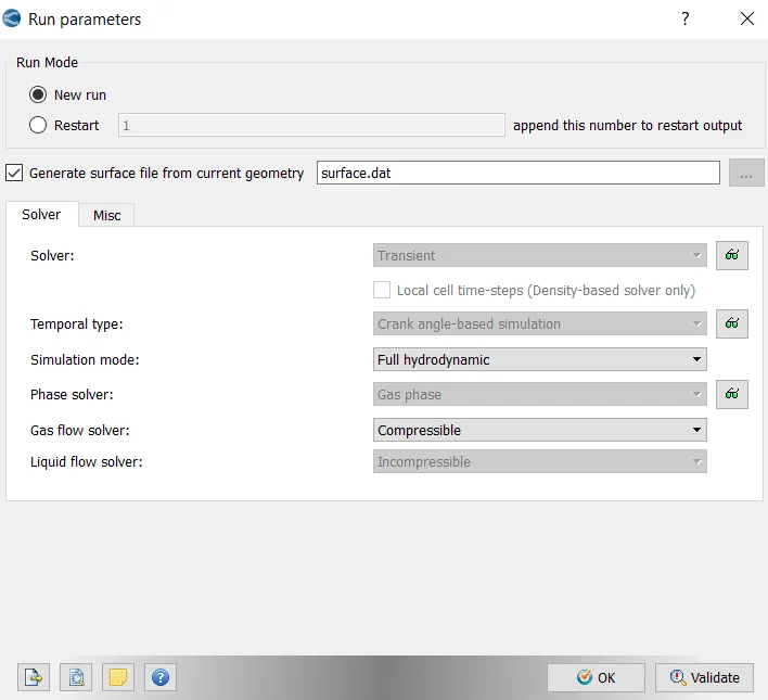
Run Parameters

Simulation Time Parameters

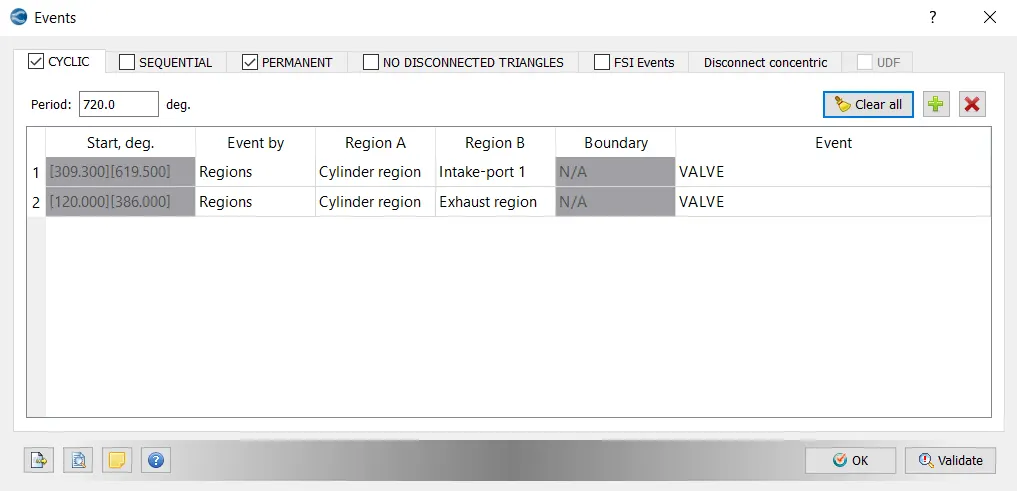
Events:

The events are created between Intake , cylinderand exhaust region as given imported valve profile data.

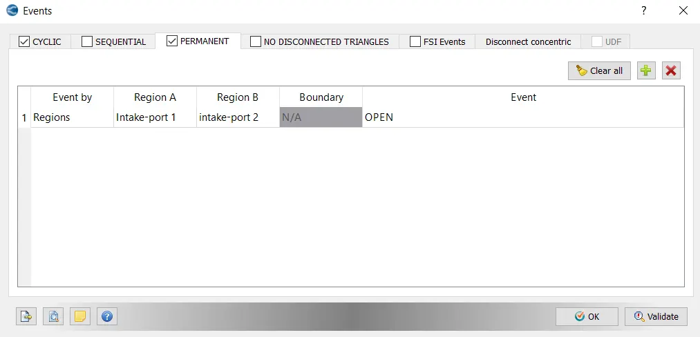
The permanent event between intake port 1 and 2 are created.

Combustion equation of Isooctane :
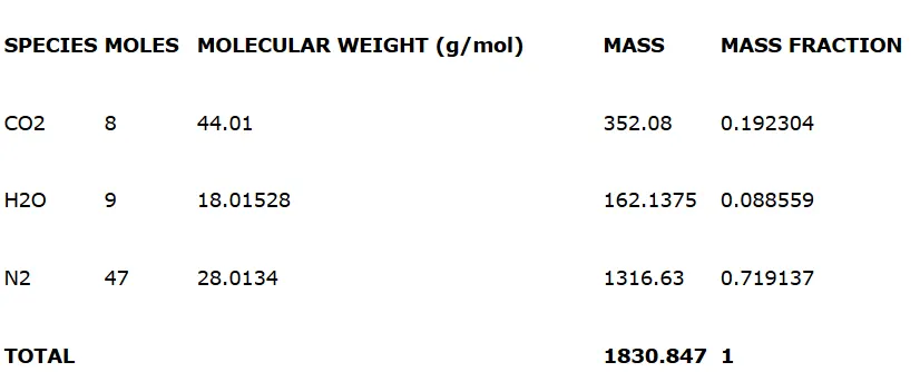
C8H18 + 12.5 CO2 + 3.76 N2 8 CO2 + 9 H2O + (3.76*12.5) N2
Fuel Calculations :
RPM = 3000 rpm
Fuel mass/cycle = 3.00 E-05
RPS = 50
DPS = 18000
Time per Degree = 5.55556E-05 s
Time per 720 Degrees = 0.04 s
Fuel Flow rate = 7.5 E-04 kg/s
We assume that the combustion is stoichiometric and the combustion products mass fractions are calculated
Stoichiometric Calculation

BOUNDARY CONDITIONS:

Inflow Boundary

Intake Port – 1

Intake Port – 2

Intake Valve Top

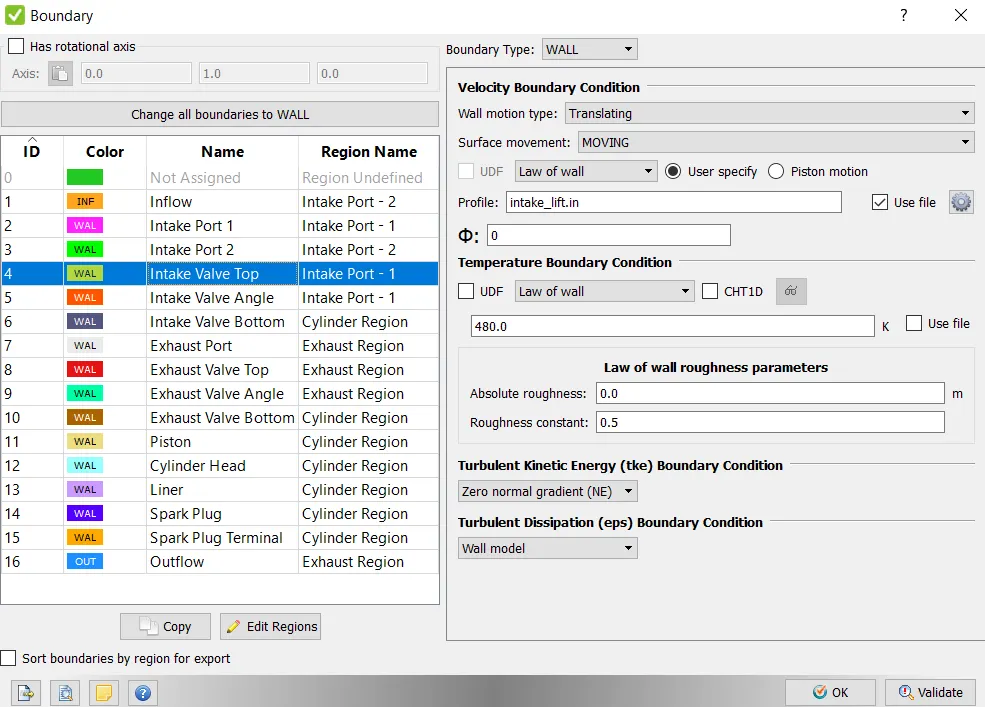
Profile Configuration of intake valve

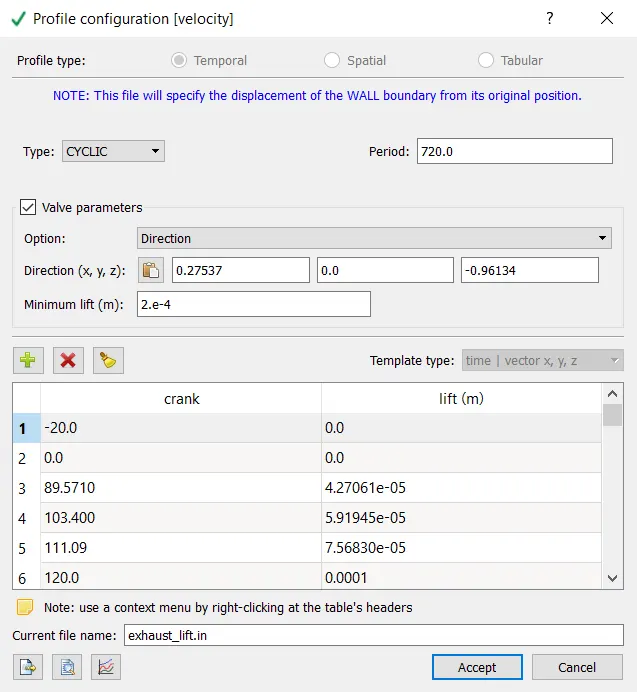
The profile configurations of intake and exhaust valves are given and this file is used. The min lift is kept as 2e-4 m and it is cyclic.

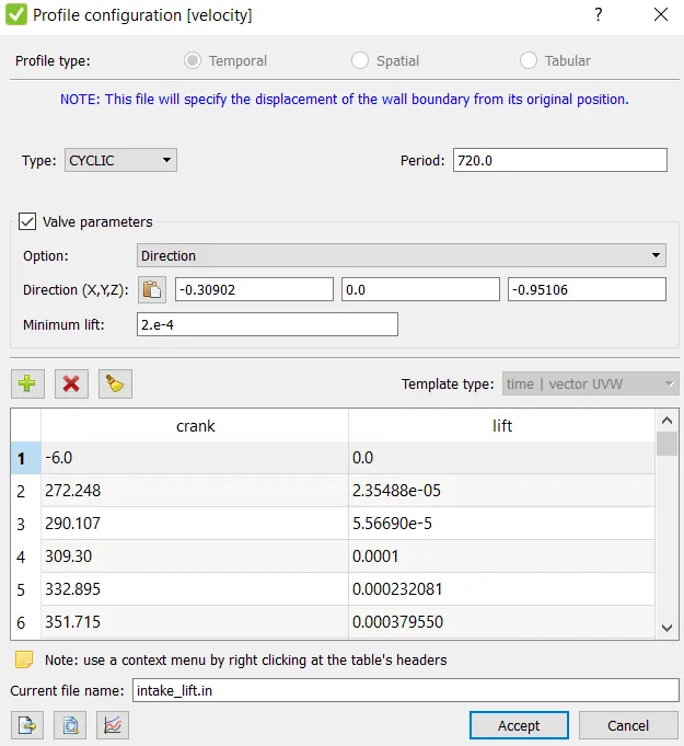
Intake Valve Angle

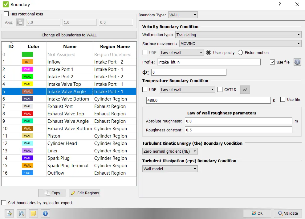
Intake Valve Bottom

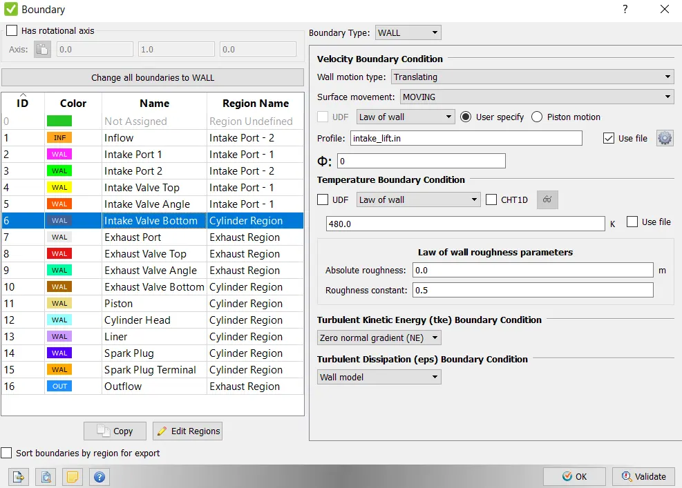
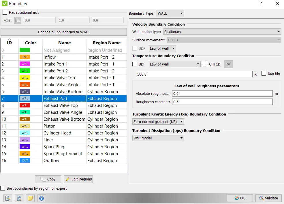
Exhaust Port

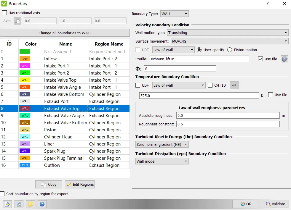
Exhaust Valve Top

Profile Configuration of exhaust valve

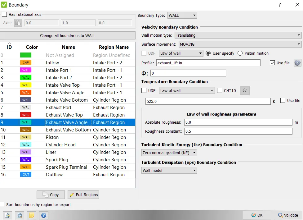
Exhaust Valve Angle

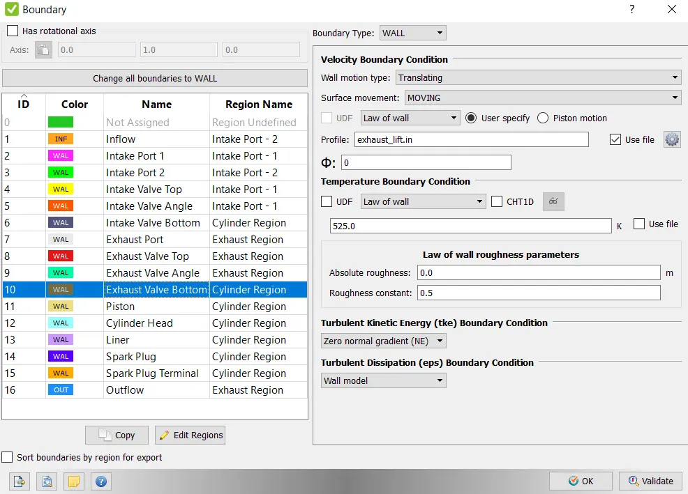
Exhaust Valve Bottom

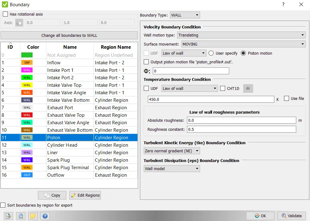
Piston

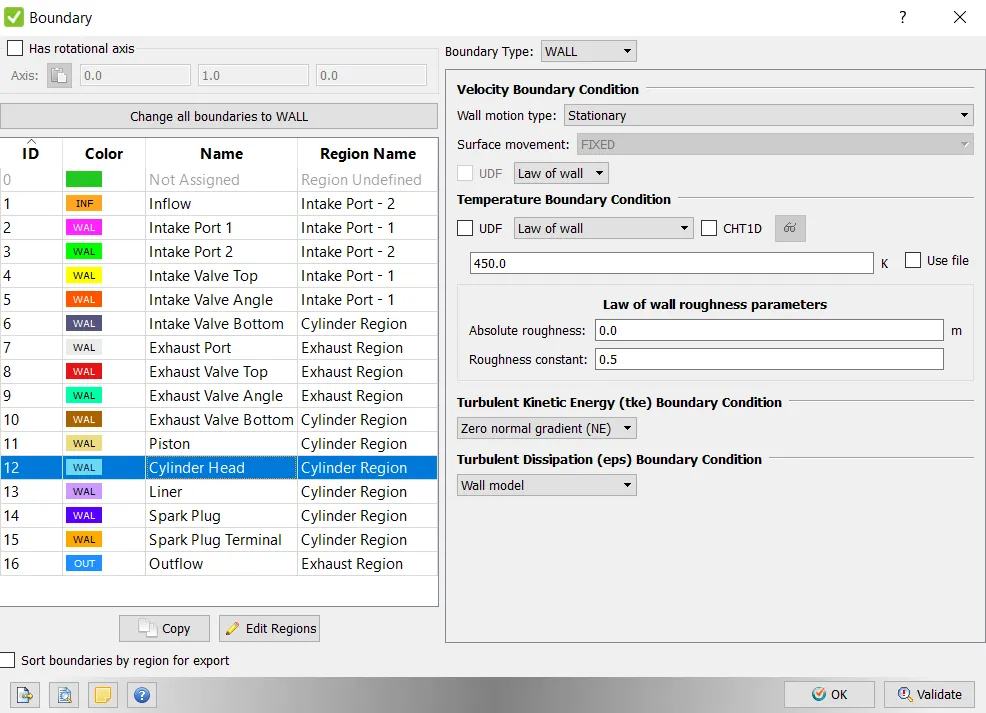
Cylinder Head

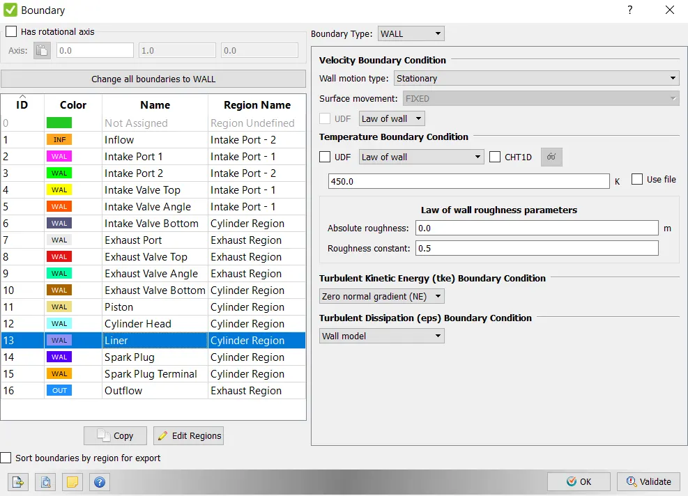
Liner

Spark Plug

Spark Plug Terminal

Outflow

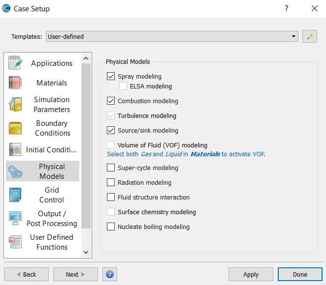
Physical Models:

Turbulence Modelling

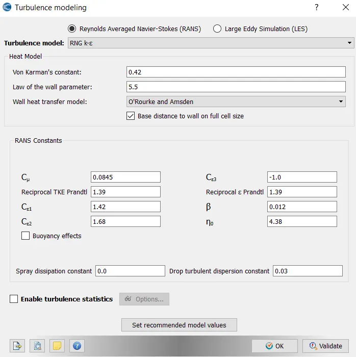
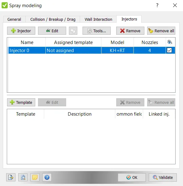
SPRAY MODELLING:

The spray model, combustion model and source/sink models are selected and it is attributed one by one.
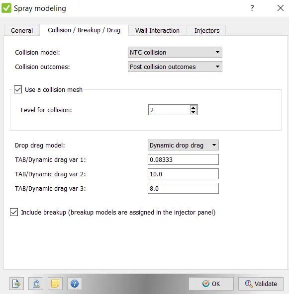
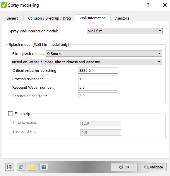
From the given parameters, the fuel injection mass is to be found out and it should be given as input. Fuel sprays breaks up into several parcels and we have to account those phenomena while defining the spray characteristics.

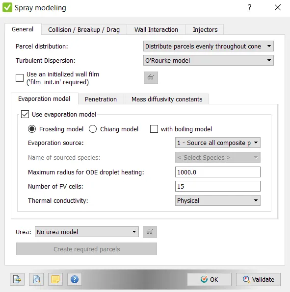
O’Rourke model in Turbulent Dispersion is for Gasoline and it used to analyse how turbulence affects droplet characteristics.
Use evaporation model is enabled because to capture the rate at which the parcel radius is going to change.
Maximum radius for ODE droplet heating is given as 1000. Here outside the sphere it is hotter and inside it is less hot due to temperature distribution. So the sphere is discretised into cells and the 2D heat equation is applied to solve it. In case of small sphere, entire sphere has same temperature and it is reasonable. But in case of bigger sphere, there will be temperature gradient. So, outside the radius ODE is solved and inside it is not solved.
Urea model is not used because it is used for exhaust after treatment system which is beyond the scope of this simulation.

Nozzle Positions :
Nozzle diameter = 250 micro-meter
Circular injection radius = Nozzle radius
Spray cone angle = 10
• Nozzle 0
o center 0.0823357 0.00100001 0.07019
o Align Vector -0.732501 0.210489 -0.647408
• Nozzle 1
o center 0.0823357 -0.00099999 0.07019
o Align Vector -0.732501 -0.210489 -0.647408
• Nozzle 2
o center 0.0823357 -0.0004 0.07019
o Align Vector -0.5 -0.2 -0.647408
• Nozzle 3
o center 0.0823357 0.0003 0.07019
o Align Vector -0.5 0.2 -0.647408

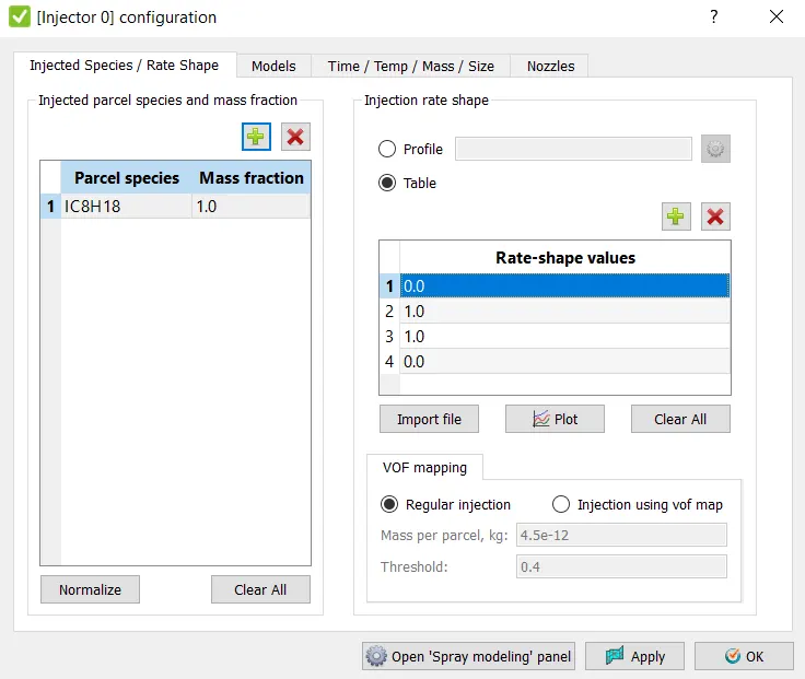
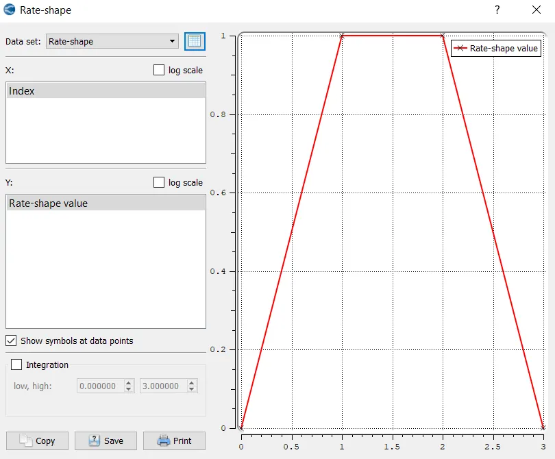
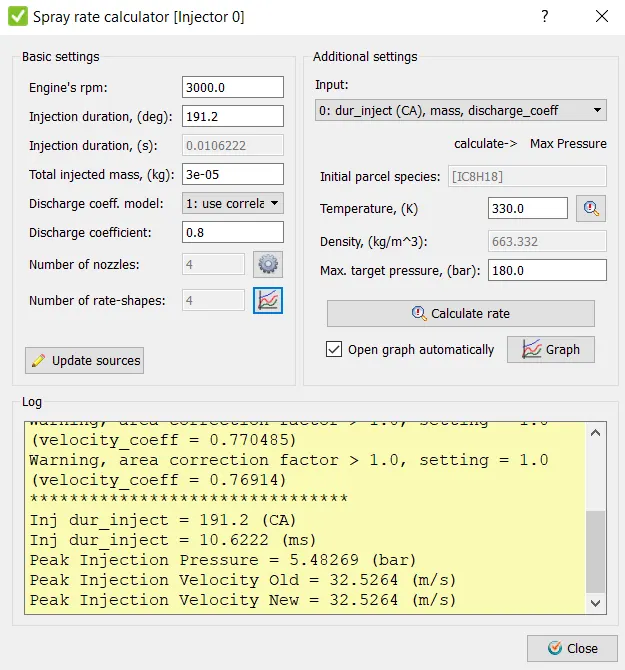
Here, Isooctane (IC8H18) is added and its mass fraction is 1. The Rate shape values are given to form the trapezoidal profile. The peak injection pressure can be found out using Tools → Spray rate preview → Calculate rate.

Injector:

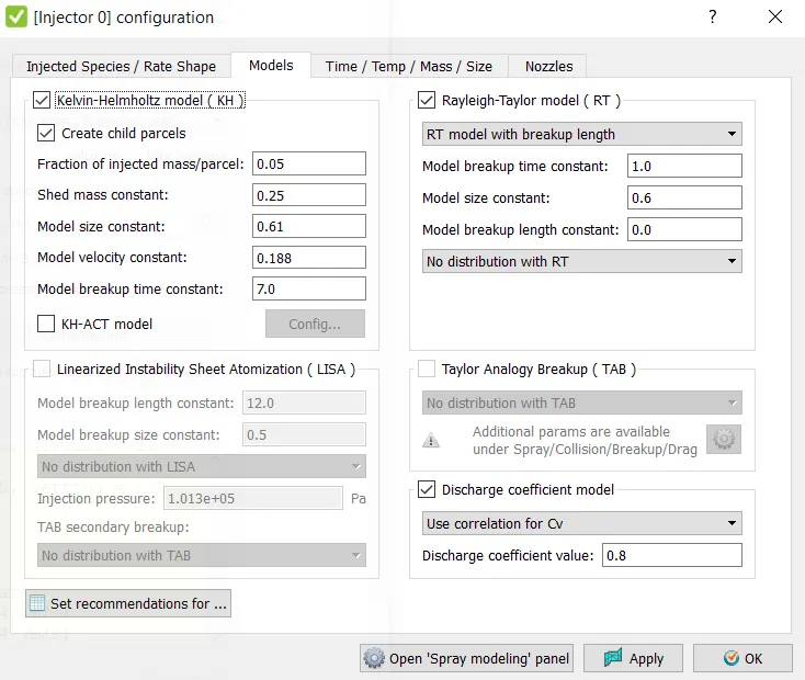
Rayleigh-Taylor model (RT) is used for solid cone sprays – gasoline and diesel.
Discharge Co-efficient model is selected and the value is given as 0.8.
The stability equation (or) dispersion equation gives us the time taken for the disturbance of the particular parcel to make it unstable.
Model size constant is used to scale down original child droplet.
Then the Set recommendations is selected Gasoline PFI is chosen.

Injection Parameters :
1. Fuel flow rate = 7.5e-4 Kg/second
2. Injection start time = -480.0
3. Injection duration = 191.2
4. Fuel temperature = 330K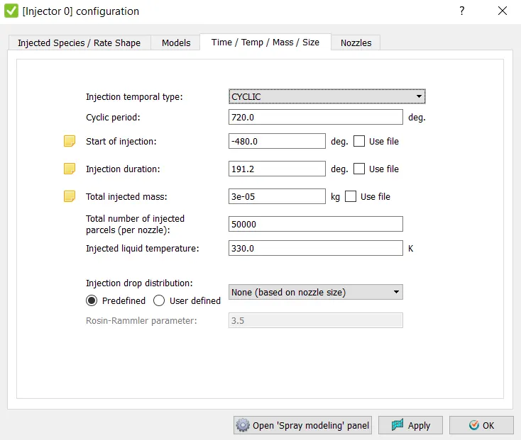

The start of injection and injection duration is given by the manufacturers. Injection takes place only at specific times and single value of mass flow rate does not have sense and mass value should be absolute. For 4-stroke engine injection takes place every 720 degrees. So for every 720 degrees, there is a particular amount of time for fuel to inject. That time is to be taken.

Calculation :
RPM = 3000 rpm => RPS = 50 rps => Degrees Per Second (DPS) = 18000 degrees/s
Time per Degree = 5.55556E-05 s => Time per 720 Degrees = 0.04 s
Fuel Flow rate = 7.5 E-04 kg/s
Fuel mass/cycle = (Time per 720 degrees) * (Fuel Flow rate) = 3.00 E-05 kg
Therefore, the Total injected mass = 3 e-5 kg

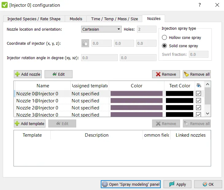
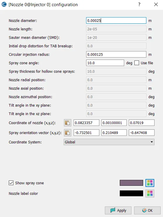
Here, four nozzles are added from Nozzle 0 to Nozzle 3. For each Nozzle the configurations are done as shown in the above figure. All the parameters listed above are given previously and it should be done for all the nozzles.

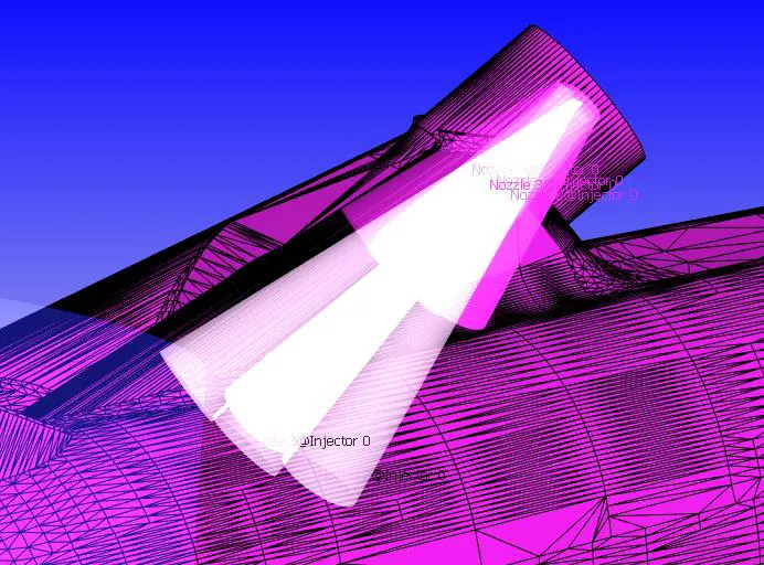
Nozzles are validated to check whether they are inside the computational domain. It is done in Spray Modelling window, Tools → Validate nozzle locations.

SOURCE/SINK MODELLING:

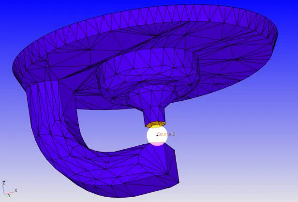
For setting up the spark, an energy source is introduced and it serves as the spark plug. By the energy equation, the energy source increases the temperature of the species. And in the species transport equation, this energy is introduced. Thus, the source term in the equation is responsible for the combustion to occur and its chemical kinetics affects the heat release, products release for every cycle. Hence this concentrated energy source is to be introduced right at the compression stroke for optimum combustion and the Source/Sink modelling is used.

Spark Ignition Parameters :
• Start of spark = -15 deg
• Spark duration = 10 deg
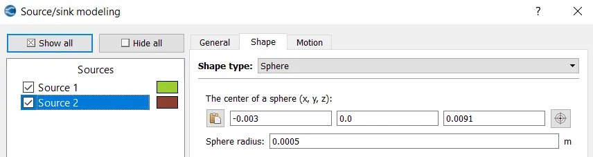
• Spark location = -0.003 0 0.0091
• Spark radius = 0.0005m

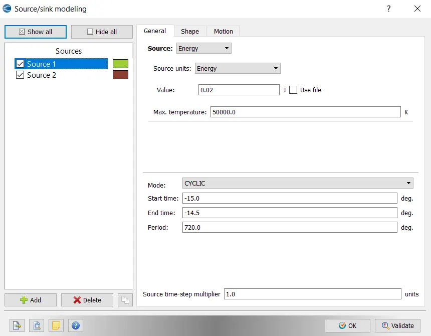
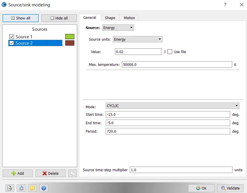
For source – 1, the energy value is given as 0.02 J and in Source – 2 also the energy value is 0.02 J during the start time (at -15 degrees). Therefore the total is 0.04 J and it lasts for 0.5 degrees (upto -14.5 degrees) in a total of 10 degrees. Then the energy from Source – 1 is shut off and the Source – 2 (0.02 J) is continued for the entire 10 degrees (upto -5 degrees).

COMBUSTION MODELLING:

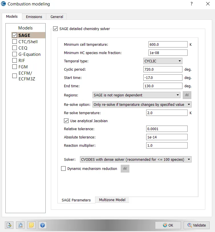
Here, the SAGE model is used and the input parameters are shown in the above figure. The combustion start time should be few degrees before spark starts (at -15 degrees spark starts). The combustion end time is determined by the degree at which the exhaust valve opens. It is done by referring the exhaust valve profile.

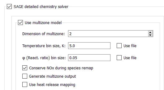
The Multizone model tab near the SAGE Parameters tab is clicked and the Use multizone model option is checked for enabling faster combustion.

Grid Control

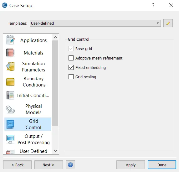
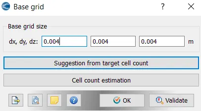
Base Grid Size

Fixed Embedding Part 1:

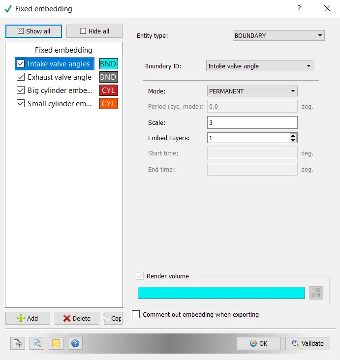
Intake Valve Angles

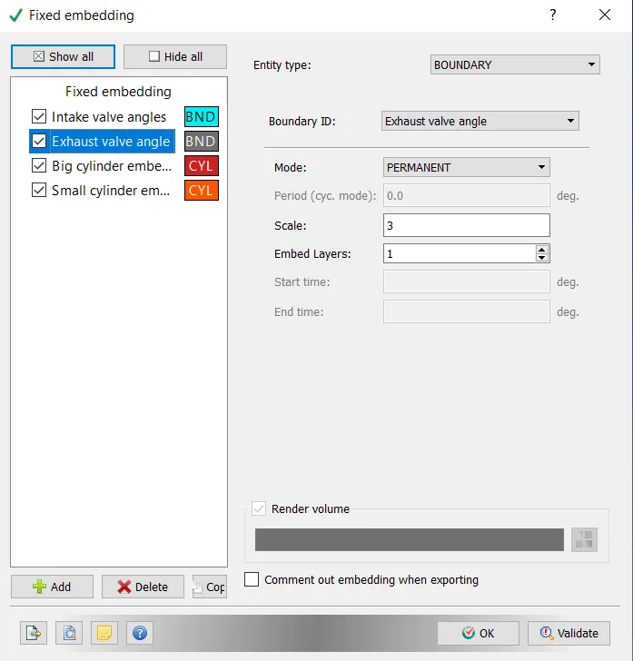
for the Intake Valves, the Boundary type embedding is used. The embedding is used to get the refinement near the intake valve angles and the Boundary ID is given the same. The scale is 3 and the mesh size here will be 0.0005 m. It is fixed and the same for exhaust valves also

Exhaust Valve Angles

Big Cylinder Embedding

Small Cylinder Embedding

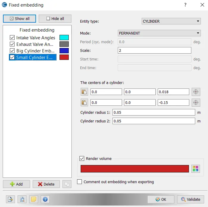
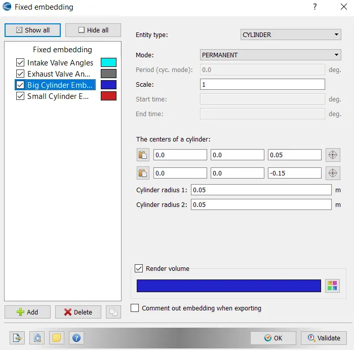
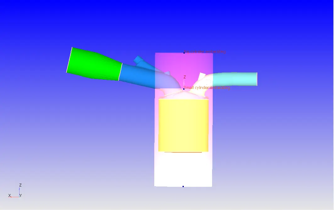
To capture the combustion precisely, the combustion chamber (Cylinder – Boundary) is made with the Cylindrical embedding. The small and big cylinders are used with the mentioned sizes with a scale of 1 and 2 with mesh sizes 0.002 m and 0.001 m respectively

Cylinder embedding

Fixed Embedding part:2:

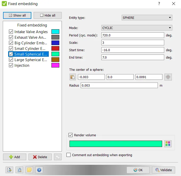
Small Spherical embedding – Spark

Large Spherical embedding – Spark

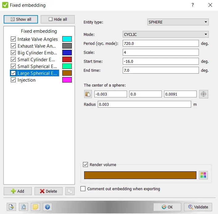
the Spherical embedding for precisely capturing the physics when the spark occurs. The small and large spheres are embedded with the scale 3 and 4 and the mesh sizes will be 0.0005 m and 0.00025 m respectively for the maximum coverage of gradient during the ignition and combustion process.

Injector embedding

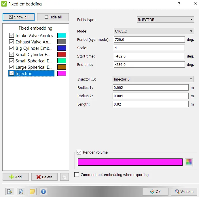
For injection, the Injector type embedding is used. The Injector 0 is the Injector ID and the Radius 1, 2 and Length are given. The scale is 4 so the mesh size will be 0.00025 m.

ADAPTIVE MESH REFINEMENT:

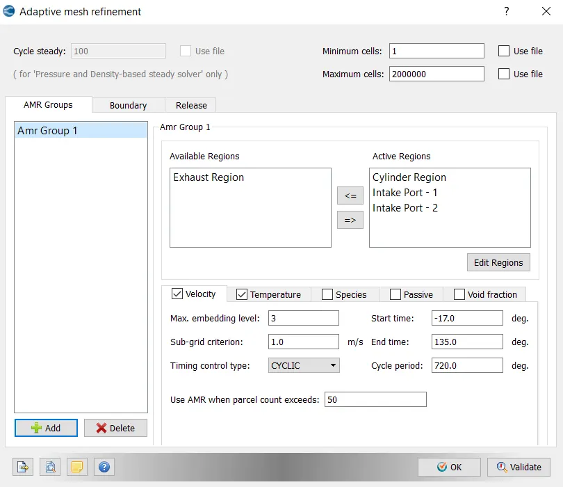
For the regions – Cylinder, Intake port – 1 and 2, the Velocity AMR is used. The start time, end time and Cycle period are as mentioned in the above figure. The maximum cell count is 2000000 cells.
The Velocity AMR works as follows :
Max Embedding Level = 3
Converge uses Octry data structure and the formula for refinement:
Grid size = Base grid / 2embedded-level
50
Here the embedded level is 3 and the refinement is as follows,
Grid size = 0.004 / 23
= 0.004/ 8
Grid size = 0.0005m
Hence the smallest grid size in this simulation will be 0.0005 m
The Sub-grid criterion (SGS) used here is 1 m/s. Therefore for change in fluid velocity of 1 m/s in the mentioned regions the mesh is refined.

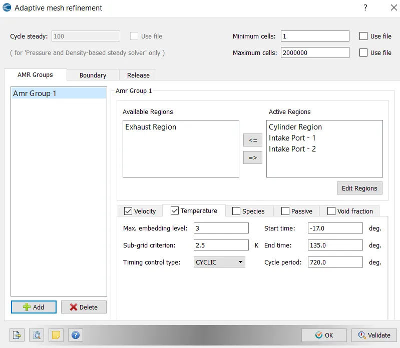
For the regions – Cylinder, Intake port – 1 and 2, the Temperature AMR is also used. The start time, end time and Cycle period are as mentioned in the above figure. The maximum cell count is 2000000 cells.
51
The Temperature AMR works as follows :
Here the embedded level is 3 and the refinement is as follows,
Grid size = 0.004 / 23
= 0.004/ 8
Grid size = 0.0005m
Hence the smallest grid size in this simulation will be 0.0005 m
The Sub-grid criterion (SGS) used here is 2.5 K. Therefore, for change in fluid temperature of 2.5 K in the mentioned regions the mesh is refined.

Model coloured by regions

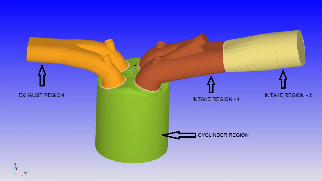
Finally, the case setup was finished and the input files are exported to the working directory. This complete PFI engine model cannot be indulged into simulation using normal computers with 4 core – processors. It takes lot of computational time to solve this model completely and this requires super computers like workstations with about 16 core – processors. Hence, the extracted input files are given to the course instructor who has the previously mentioned supercomputer. The simulation was run by them and the output files were shared. From that the 3D output files are generated using Converge Studio and the results are post processed using the line plots from studio and 3D plots using ParaView. Results are shown in the following section. By the end of this report, the link to the animations are provided. Several parameters like velocity, temperature, pressure and other quantities are animated using ParaView.

Results:

Mesh:

X-normal

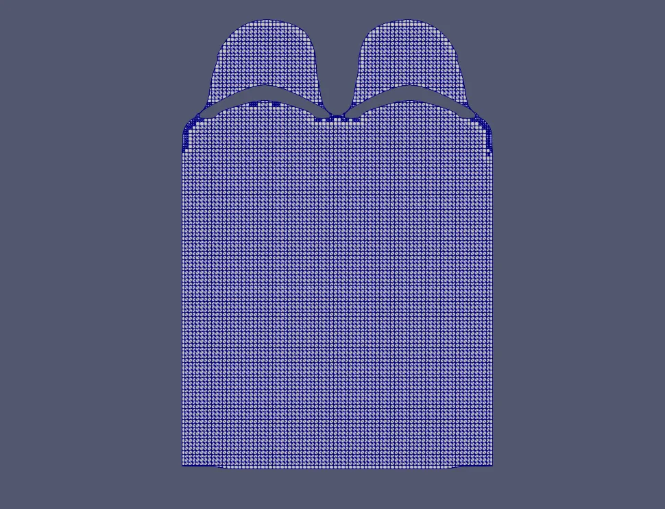
z-normal

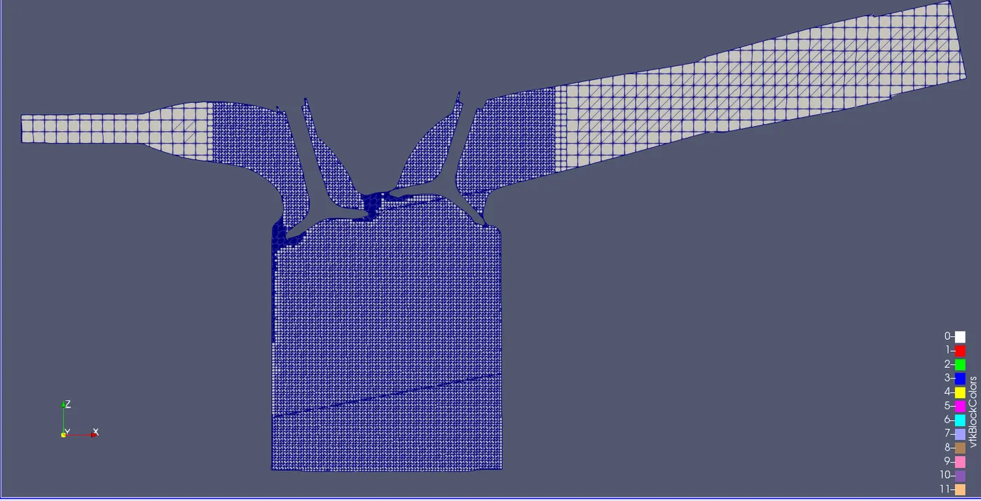
The 3D animation of simulation:

The Temperature animation:

CONCLUSION:

In conclusion, Computational Fluid Dynamics Software – Converge Studio, was a useful method to simulate the fluid flow behaviour with the relevant governing equation. The SI8 PFI Engine was successfully simulated using the given conditions and specifications. The finer mesh size could provide the accurate results but, it increases the computational time tremendously. So, tools like fixed embedding and adaptive mesh refinement were used to refine the mesh wherever and whenever necessary. The physical models for capturing the combustion, sprays, sparks and turbulence are selected appropriately for this case. To solve CFD cases like we did here, requires high computational power machines.

1. What is the compression ratio of this engine?

Generally, Compression ratio (r) of the engine is the ratio of total cylinder volume when the piston is at the bottom dead centre (BDC) = VT, to the clearance volume = VC when piston at top dead centre (TDC).
r = VT / VC
r = (VC + VS) / VC , where VS is the swept volume.
The compression ratio of our engine is found using the volume plot show below i.e, by the ratio of maximum volume to the minimum volume.

Volume Plot :

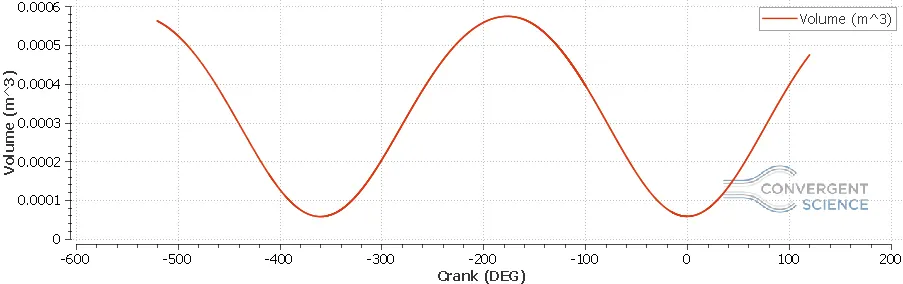
Maximum Volume = 0.00057 m3
Minimum Volume = 5.75 * 10-5 m3
Therefore, compression ratio (r) = Maximum Volume / Minimum Volume
= 0.00057 / 5.75 * 10-5
Compression ratio (r) = 9.9 : 1

2. Why do we need a wall heat transfer model? Why can't we predict the wall temperature from the CFD simulation?

Generally, the operation of an IC engine is based on chemical reactions taking place during the combustion. During power stroke, the fuel-air mixture gets ignited (incase of spark ignition engine) by the spark plug and chemical reactions takes place inside the combustion chamber. These reactions raise the temperature inside the chamber and forces the piston to expand. During this process there will be an energy interaction between the fluid and the walls i.e, surfaces of the IC engine in the form of heat. The heat transfer between the fluid and solid surface takes place generally in two modes – convection and radiation. In general case CFD simulation, the Navier – Stokes equation is solved to get the results of the fluid flow. To get accurate results, mesh size should be less and it increases computational time.
For this PFI engine simulation it takes lot of time to compute the case as it involves a complex geometry and processes. If we want to capture the heat transfer – especially convection of heat from fluid to the solid surface, energy equations should also be solved. This increases the time of simulation. For radiation of heat from the solid surface to atmosphere, an external mesh is to be made to depict the external atmosphere and to solve the energy equation which increases the cell count. It makes the simulation to run forever. Hence, we use conjugate heat transfer model where the solid part is solved in a steady state using super-cycling option and the fluid part is solved in transient case.
For simulating complex geometries like IC engines, it takes lot of time for computing the fluid part itself in transient case along with the combustion and reaction processes. So it becomes difficult to predict the wall temperature from the CFD simulation as solving of heat transfer along with the Navier – Stokes equation consumes lot of computational power and time. Wall heat transfer models are used to approximate this case. Basically, all the physical models used in a CFD simulation uses some approximation to minimize computational time. Wall heat transfer models are used if we are focused only on heat transfer giving less importance to fluid motions and reactions. For efficient operation of engine, the walls should be maintained at a certain temperature. This is achieved by pumping coolant to take away the excess heat from cylinder wall.

3. Calculate the combustion efficiency of this engine.

Combustion efficiency is a measure of how effectively the heat content of a fuel is transferred into usable heat. In other words combustion efficiency is the ratio of output energy derived from the engine to the input energy provided to the engine during the combustion process.
Output Energy = 1241 J
Mass of fuel used per cycle = 3 * 10-5 kg
Lower Heat value of fuel (IC8H18) used = 44.8 MJ/kg
Potential energy in the fuel i.e, input energy = 44.8 * 10 6 * 3 * 10-5 = 1344 J
Combustion efficiency = Output energy / Input energy
= 1241 / 1344 = 0.9233
Combustion Efficiency of this engine = 92.33 %

4. Use the engine performance calculator, to determine the power and torque for this engine.

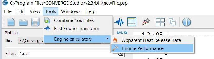
The engine performance calculator is used to analyse physical data and get useful results from the data. It is an useful tool to calculate the quantities need to define an engine. In our case the calculator is opened and the file – thermo_region.out file is added for the cylinder and then the engine.in file is loaded which contains the bore and stroke of the engine.

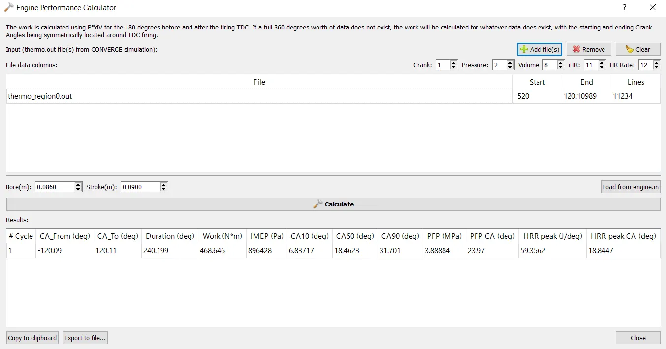
Duration of combustion = 240.199 degrees
Work done = 468.646 Nm
Indicated Mean Effective Pressure (IMEP) = 896428 Pa
CA 10(deg) = 6.83717 degrees
CA 50(deg) = 18.4623 degrees
CA 90(deg) = 31.701 degrees
Power is the rate of work done i.e, the amount of work done per unit time.
Power (P) = Work done / Time

We know that, Time per Degree = 5.55e-5 s
Therefore, for one cycle of operation time taken (t) = 240.199 * 5.55e-5 = 0.013331 s
Power (P) = Work done / Time = 468.646 / 0.013331= 35154.48 J/s (or) 35154.48 W
Power (P) = 35.15 KW

Since Work and Torque has the same unit (N-m) , it doesn't mean value for Torque and Work will be the same. Both are different quantities and has totally different meaning. So the value for work got from the engine performance calculator is not the value for the torque. The Torque is calculated from the formula,

Power(P) = (2 * π * N * T) / 60
Torque (T) = (P * 60) / (2 * π * N)
The crank speed (N) = 3000 rpm – given at the beginning.
T = (35154.48 * 60) / (2 * π * 3000)
Torque (T) = 111.9 Nm

5. What is the significance of ca10, ca50 and ca90?

The values CA10, CA50, CA90, represents the Crank Angle at the completion of 10%, 50%, 90% of combustion. From these values we can infer the time taken for the evaporation and combustion of the fuel. If the combustion process is fast, which requires few crank angles and leads to increase in emissions. CA10 represents the start of ignition, CA50 represents the end of fuel-air mixture combustion and at CA90 the burning of unburnt fuel is done by the propagating flame. If CA90 value is large, the crank angles taken increases and the exhaust stroke tends to push the premature combustion products.