Week 10: Project 1 - FULL HYDRO case set up (PFI)

Introduction: IC engines are complicated machines that are extremely sophisticated when it comes to their design. Normally before any engine is approved for public usage, a lot of testing has to happen before it goes for production. The experimental testing highly costly and also takes long time. Therefore computer simulations are used to obtain approximate results that are more or less equal to the values that are obtained experimentally. These reduce a lot of time and are very less expensive. According to the results that are obtained, changes are made once again the design of the engine and it is simulated once again. This process is repeated untill the most feasible design is obtained.

Purpose of running the nohydro case: No hydro case is extremely necessary especially to look at how the mesh is changing from time to time. Because if there is no such option, we have to run the entire full hyro case which takes a lot of time to complete. Thus the mesh parameters, events and other conditions such as embedding can be looked into carefully by performing the nohydro simulation.

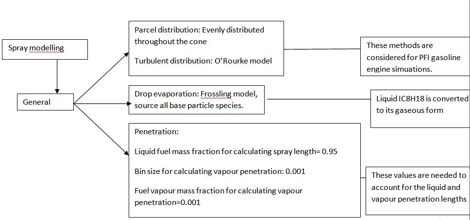
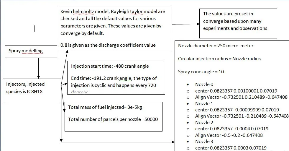
Spray modelling: Spray modelling is nothing but having the effect of fuel spray in the computationa simulation of IC engines. Spray models are used because this reduces the computational time significantly else we have to perform multiphase simulation which consumes a lot of time. This is just an approximation which means that the effect of sprays is represented in this fashion.

Some terminologies of spray modelling:

1) Primary breakup: Splitting of drop from main stream.

2) Secondary breakup: Splitting of primary drop into multiple drops.

3) drop drag: The drag experienced by a drop due to the air resistance is called drop drag.

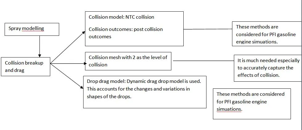
4)Collision and coalescence: Collision of two or more drops and formation of new drop.

5) Turbulent dispersion: Transport of mass, momentum and heat etc due to random motion of the parcels and drops.

6) Evaporation: Evaporation of drops into vapour. Frossling and chiang models are present in converge for evaporation.

7) Collision:We need to make use of the collision mesh in order to obtain the collision of the drops properly. The default values in converge are used.

8) Drop drag: Spherical drop drag and dynamic drop drag model are present in converge. Spherical model assumes that the drops as spheres whereas dynamic model accounts for changes or variations in drop shape. It uses TAB model to determine the drop distortion.

9) Drop wall interaction: When a drop strikes a wall, the drop can split, or reflect off or stick to the wall. These type of effects are modelled using O'Rourke or Kuhnke model.

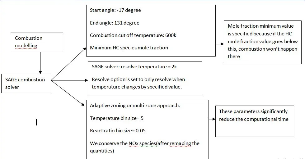
Combustion modelling: In this simulation, SAGE combustion solver is used. SAGE is a combustion solver that uses the principle of chemical kinetics to solve for the reaction rates of various species. Arhenius principle is used in the backend to solve for the reation rates of various reacting species. This solver calculates the heat released which is used as a source term in fluid equations. chemical kinetics ODE's of various species are solved using CVODES and the values obtained are used to solve the species transport equations.

Acceleration tchnique: Normally computing the values at each and every zone is extremely time consuming and therefore SAGE solver uses something called multizone method. This means that all the cells in the regions where the combustion takes placed are grouped into bins. The bins are created based on temperature and equivalence ratio of fuel and air. All the cells that have the same values of equivalence ratio and temperature will have the same combustion results. Therefore as a result of clustering the cells into bins, the combustions solver solves the entire bin instead of each cell, thus significantly reducing the computational time.

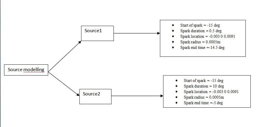
Source modeling: Spark plug is modelled as a source of energy that activates just before start of the combustion. The energy is included in the fluid flow energy equations.

Case setup:

Boundary flagging is done appropriately first. After boundary flagging is done, surface repairs are done to repair the open edges, intersections, manifold edges, norma orientation errors and other errors.

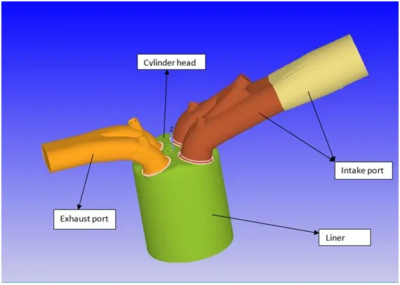
The boundary flagging with respect to different regions.

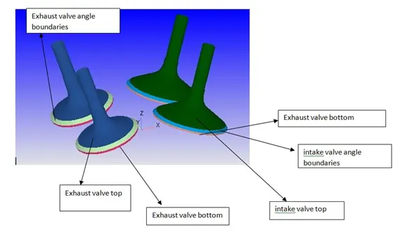
The intake and exhaust valves are divided into three boundaries each. They are top, bottom and angle boundaries of the intake and the exhaust valves.

Boundary conditions:

Boundary	Type	Motion type	Details	Temperature/Pressure
Piston	Wall	translating	piston motion	T=450.0K
Inflow	inflow	NA	species:Air	P=101325Pa, T=363K
Liner	Wall	stationary	NA	T=450K
Cylinder head	wall	stationary	NA	T=450k
exhaust port	wall	stationary	NA	T=500K
Outflow	outflow	NA	species: CO2,H2O,N2	T=800K
exhaust valve top	wall	moving	exhaust_lift.in motion profile	T=525k
exhuast valve angle	wall	moving	exhaust_lift.in motion profile	T=525k
exhaust valve bottom	wall	moving	exhaust_lift.in motion profile	T=525k
intake port 1	wall	stationary	NA	T=425K
intake valve top	wall	translating	intake_lift.in motion profile	T=480k
intake valve angle	wall	translating	intake_lift.in motion profile	T=480k
intake valve bottom	wall	translating	intake_lift.in motion profile	T=480k
spark plug	wall	stationary	NA	T=550k
intake port 2	wall	stationary	NA	T=425k
spark plug terminal	wall	stationary	NA	T=600k

`C8H18 + 12.5(O2 + 3.76N2) -> 8CO2 + 9H2O + 47N2`

This is the reaction of

Species mass fraction in the cylinder region and exhaust region:

Species	Moles	Molecular weight	Mass	Mass fraction
CO2	8	44	352	0.192349727
H2O	9	18	162	0.719125683
N2	47	28	1316	0.0885249
Total	64	90	1830	1

Regions and Events: Regions are the different fluid or solid volumes that are divided according to the need of the simulation.Events are used to control the interaction between two different regions. During any time if we do not want the regions to interact with each other(that is there should not be any flow between the two regions), disconnect triangles are formed by the solver that prevent any flow between one region to another.

Regions	Temperature	Pressure	Species	boundaries
Intake region1	390.0	101325.0	IC8H18 O2 N2	intake port1 intake valve angle boundaries intake valve top
Intake region2	370.0	101325.0	O2 N2	inflow intake port2
Cylinder region	1360.0	185731.0	CO2 H2O N2	piston liner cylinder head exhaust valve bottom intake valve bottom spark plug spark plug terminal
Exhaust region	1215.0	103737.0	CO2 H2O N2	exhaust port outflow exhaust valve top exhaust valve angle boundaries

Spray modelling:

Adaptive mesh refinement:

This techniqque is used to refine the mesh either cyclically, sequentially or permanently. This technique is based upon refining the mesh depending upon the curvature(second derivatives) in the field variables such as temperature, velocity etc.

This technique automatically increases grid resolution based on the second derivatives of the field variables. They are activated on region to region basis. At each and every time step and at each and every computational mesh cell, the value of `phi'` which is equal to `(d^2phi)/dx^2 (deltax^2)/24` is computed. This value is the sub grid scale value of the field vector `phi'`. This `phi'` can be temperature, velocirty pressure etc. If the value of `phi'` at any computational cell gets lesser than the specified SGS value, the size of the cell becomes `(base grid size)/2^n` where n is the scaling level.

`phi'= phi-barphi` where `phi`is the theoretical value. `phi'` is the sub grid scale value and `barphi` is the value obtained by computational calculation by the solver. So if the cell size reduces, the `deltax`value reduces and hence the value of `phi'`reduces. It means that the computationally obtained value is getting closer to the theoretical value and the error between them is reducing. Hence the computational results get better and better as the refinement is increasing.

1) We do the adaptive mesh refinement in the intake region1, intake region2 and the cylinder region as the velocities and temperatures in these regions are critical in these region.

2) The mixing of air and fuel happens in the intake regions1 and 2 therefore it is critical to perform AMR for velocity and temperature.

3) In the cylinder region, the combustion takes place and hence it is important to perform AMR in this region.

4) Since there are no reactions happening in exhaust region and only the output of the combustion flows through this region, there is no need of AMR.

Types of AMR used:

1) Velocity:SGS criterion is 1 and max embed level is 3, this refinement is permanent(that means it happens throughout the simulation)

2) Temperature: SGS criterion is 2.5 and max embed level is 3, this refinement is cyclic and happen periodically every 720 degree crank angle. It starts at -17 and ends at 131 degree(happens the entire duration of combustion). This is because critical temperature fluctuations happens only during the combustion stroke.

Fixed embedding:

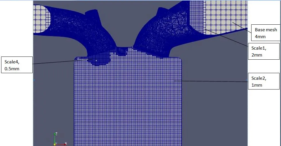
Fixed embedding also can be permanent, cyclic or sequential. Fixed embedding can be used to give further refinement to certain areas of the computational domain. In this simulation of the port fuel injection, different regions and boudaries were given different refinements and scaling factors based upon the necessity. If the scale factor given to any particular boundary or region is n, then the size of mesh on that particular boundary becomes (base grid size)/2^n. This technique is useful for refining the walls in case of aerdynamic simulations, to obtain a fine mesh in the intake and exhaust valve areas where capturing the physics of the problem is extrmely essential.

Embedding name and entity type	Mode	scale	Size after scaling= (base mesh size)/(2^n)	Notes
Intake valve angle boundaries, boundary entity type	Permanent	3	4/8 = 0.5mm	1Layer
Intake valve angle boundaries, boundary entity type	Permanent	3	4/8 = 0.5mm	1Layer
Cylinder bigger, cylinder type	Permanent	1	4/2 = 2mm	Radius = 0.05 Coordinates: 0,0,0.1 and 0,0,-0.1
Cylinder smaller, cylinder type	Permanent	2	4/4 = 1mm	Radius = 0.05 Coordinates: 0,0,0.01 and 0,0,-0.1
Smaller sphere embedding, sphere type	Cyclic period:720 degree start angle=-16 end angle= -7degree	5	4/32 = 0.125mm	Radius = 0.001 Coordinates: -0.03,0,0.0091
Larger sphere embedding, sphere type	Cyclic period:720 degree start angle=-16 end angle= -7degree	3	4/8 = 0.5mm	Radius = 0.003 Coordinates: -0.03,0,0.0091
Injector embedding, injector type	Cyclic period:720 degree start angle=-483 end angle= -283 degree	4	4/16 = 0.25mm	Radius1 = 0.002 Radius2 = 0.004 Length= 0.02

Results:

https://youtu.be/5dqN9DeyyQ8 -The animation of the temperature throughout the Port fuel.

https://youtu.be/UI5ZFtF52F4- The animation of the mesh changes throughout the Port fuel.

The mesh changes happen throughout the four strokes.The velociy adaptive mesh refinement happens throughout all the strokes whereas the temperature AMR happens only durinng the entire combustion stroke.

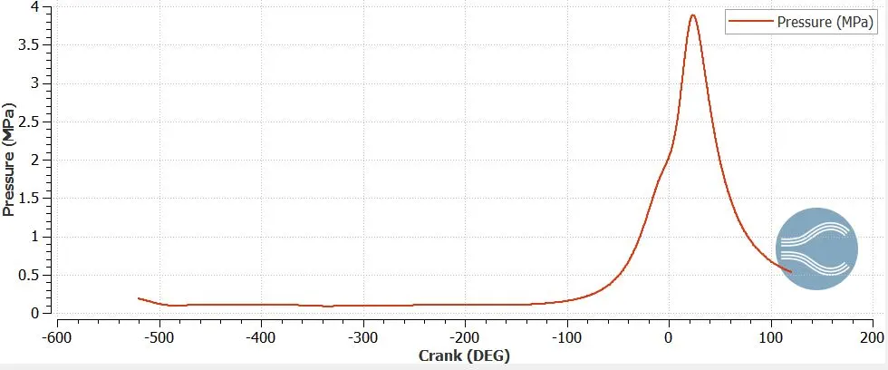
The above plot shows pressure in the cylinder region with respect to the crank angle. The simulation starts at -520 degree crank angle and ends at 120 degree. The spary starts at -480 degree crank angle, the pressure rises in the compression stroke. The pressure further rises during combustion and it reduces during the exhaust stroke.

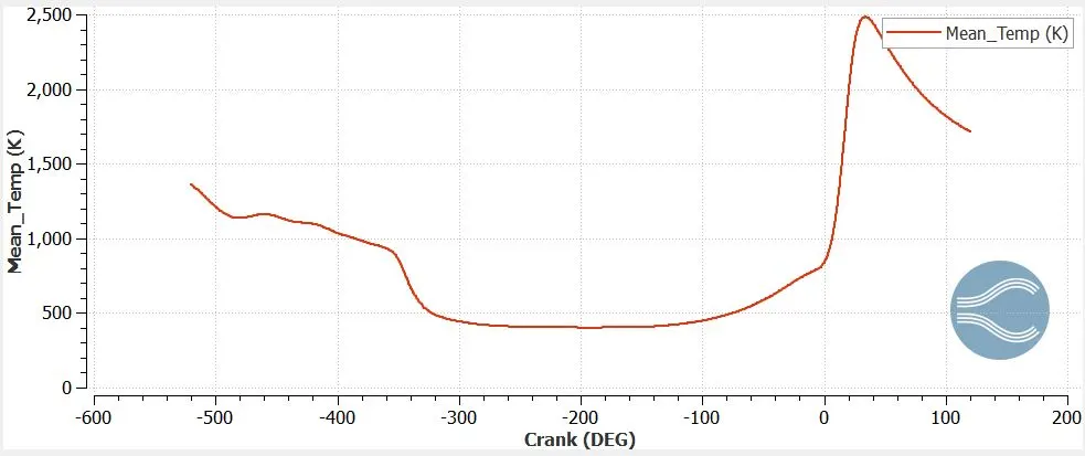
It can be seen that the temperature rises during the compression stroke and the temperature further shoots up during the comnustion stroke. The temperature of the cylinder follows a similar trend as that of pressure for the compression and combustion and exhaust strokes.

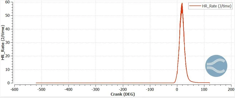
It can also be observed from the above figure that the temperature in the cylinder is at its peak temperature when there is maximum heat rejection happening in the cylinder as shown in the above two figures of temperature of cylinder and heat rejection rate of the cylinder.

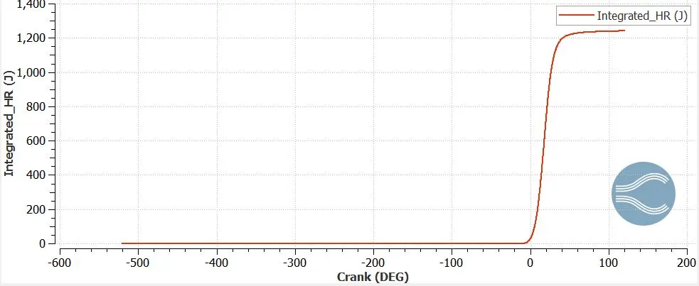
On integrating the above graph, we obtain total heat rejection for the entire duration of the simulation.

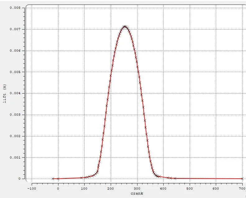
Lift vs crank angle plot for the exhaust valve

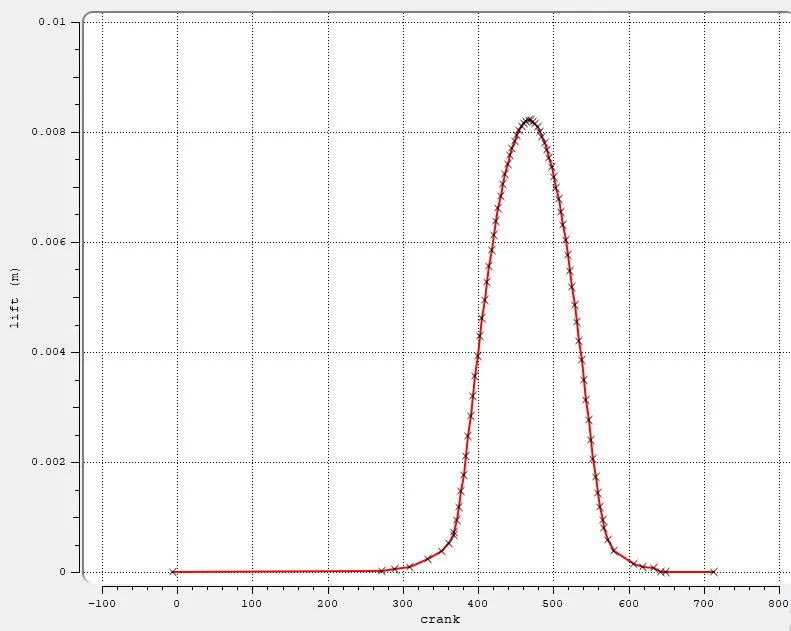
Lift vs crank angle plot for the intake valve

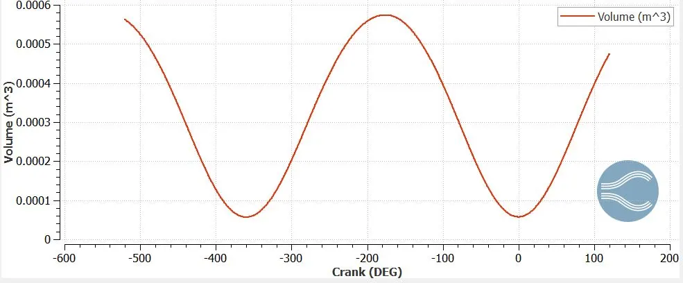
From the above animation and the volume plot, it can be seen that the spray starts at -480 degree crank( even before the piston reaches the top dead centre) thats why from crank angle of -480 to about -360, the volume of the cylinder decreases. This is because although the spray has started, the piston has not yet reached the top dead centre which means that the exhaust stroke has still not yet complete and therefore there is decrease in volume.

At about -360 degree, the intake valve starts to open and therefore the volume of the cylinder raises in the intake stroke and this happens upto -180 degree crank angle. At -180 crank angle, the piston is at the bottom dead centre and hence maximum value of volume is obtained at this position. After this the compression stroke starts and the volume of the cylinder reduces again to minimum when the piston reaches the top dead centre . Now the combustion stroke starts at -17 degree crank angle( even before the piston has reached the top dead centre) and it continue upto the end of the simulation thus increasing the volume once again.

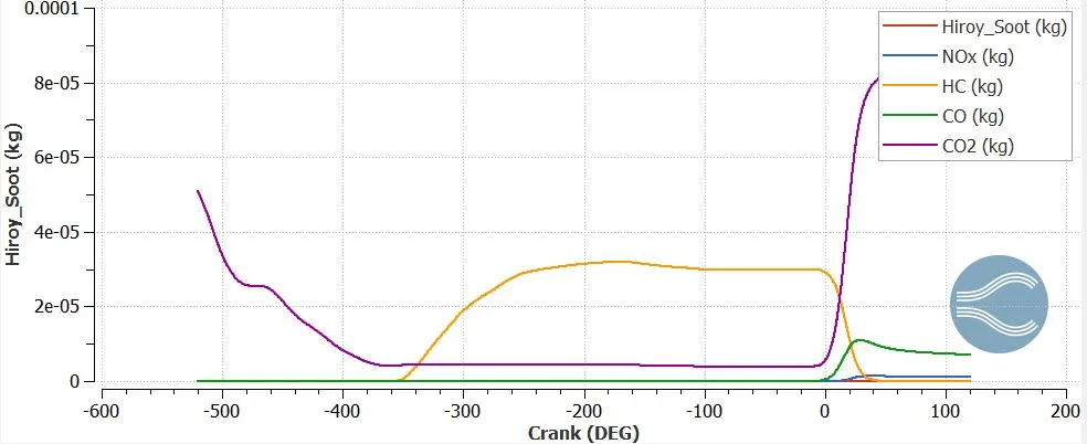
It can be seen from the above graph of the emissions of various gasses. The hiroy soot releases is in the order of 1e-8kg which is very very less compared to the other species that are released.

It can also be observed from the above graph that during the intake and compression strokes, the masses of CO,CO2,NOx are almost constant and do not change and their masses increase during the combustion stroke. This increase is because CO,CO2,NOx are end products of combustion process. Therefore their masses increase.

However the HC masses are higher during the intake, compression strokes because during these two strokes, no combustion has taken place and there is no fuel that is burnt. After the combustion has started, the fuel starts to burn, therefore the HC mass also reduces during that entire stroke.

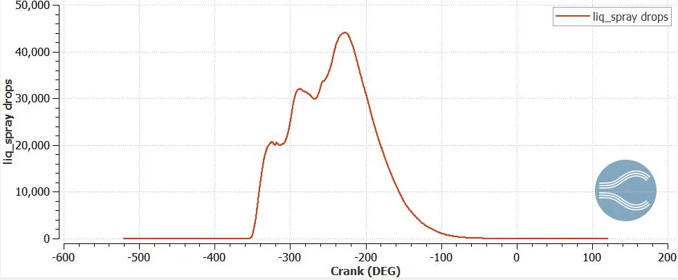
The above graph shows the variation of the number of liquid drops with crank angle in the cylinder region. The number of drops doesnt increase and remains constant from -520 degree crank until the intake stroke begins. As the compression, combustion and exhaust strokes happen, more and more amount of fuel is burnt and the number of liquid drops decreases.

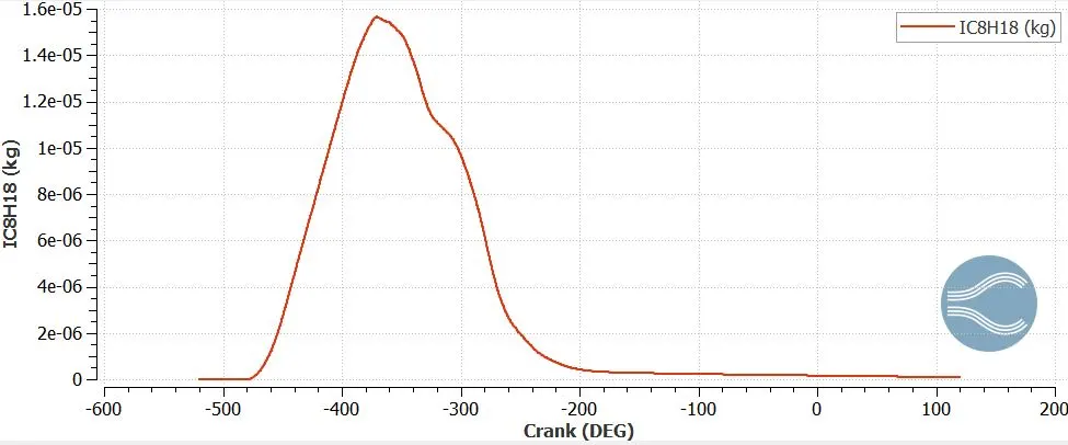
This graph shows the variation of mass of isooctane with crank angle in the intake region that is closer to the cylinder. The mass of the fuel in this region as the fuel injection begins. It raises upto the end of the intake stroke. In this region, some amount of vaporization might occur. Therefore as the compression stroke begins, intake valve would be closed and hence slowly due to little amount of vaporization in the intake region, fuel mass starts to reduce and it reaches a minimum value. This minimum value of fuel present is the trapped mass of the fuel. This trapped mass is 1e-7 and our injected fuel mass is 1e-5. The trapped mass is very negligible compared to the injected liquid mass.

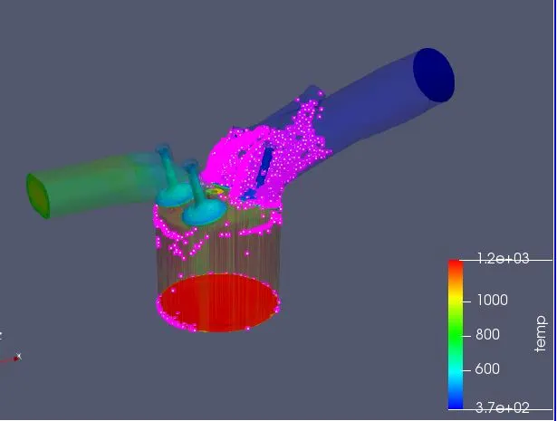
Inside the PFI cylinder at the end time of the simulation(the combustion has not yet completed)

Compression ratio:

5.70467e-5 m^3 is the minimum volume and 0.000574215 m^3 is the maximum volume. Therefore the compression ratio of this PFI gasoline engine is `(Vmax)/(Vmin)`= 10.0658.

Combustion efficiency of this engine:

Combustion efficiency of the engine is the heat released by the engine after combustion divided by the product of mass of fuel and its calorific value.

`(eta)eng = (IHR)/((mass of fuel )*(CV))`

efficiency of engine = (1240.22)*100/(3e-5*47*10e6)= 87.9%

Engine performance:

These performace parameters are obtained from a tool in converge. This tool computes the gross work, duration and various other parameters which are discussed below.

Gross work= 468.646Nm

Duration to calculate gross work= 240 degree

RPM of engine= 3000

now time in seconds to revolve 240 degrees = (240*60)/(360*3000) = 0.0134 seconds

Power= work/time = 468.646/0.0134 = 34,973Nm/s or 34,973W

Power = `(2piNT)/60`, it means T= torque = `(power*60)/(2piN)`= 111.37Nm

CA10, CA50, CA90 indicate the crank angles at which 10%,50% and 90% of the fuel is burnt.

Why do we need a wall heat transfer model? Why can't we predict the wall temperature from the CFD simulation?

A simulation which involves heat transfer between two different medium such as between a solid and fluid by means of conduction or convection phenomenon is called conjugate heat transfer simulation. In order to calculate the temperatures of various walls due to the hot fuel temperatures, we normally need to perform the CHT analysis. However for such a complicated phenomenon, performing CHT analysis would take indefinitely large amount of time. In this simulation, O'Rourke and Amsden wall heat transfer model is used. These wall heat transfer models are approximation models that are used to calculate the temperature of the walls. They save a lot of computational time.