Week - 10 Hyperelastic Material Models

Week - 10 Hyperelastic Material Models

OBJECTIVES :

To perform a tensile test with 100% strain for both Mooney Rivlin and Ogden material constants using given stress-strain data.

HYPERELASTIC MATERIALS :

For many materials, linear elastic models do not accurately describe the observed material behavior. The most common example of this kind of material is rubber, whose stress-strain relationship can be defined as non-linearly elastic, isotropic, incompressible, and generally independent of strain rate. Hyperelasticity provides a means of modeling the stress-strain behavior of such materials. Ronald Rivlin and Melvin Mooney developed the first hyperelastic models, the Neo-Hookean and Mooney Rivlin solids.

They are commonly used to model mechanical behaviors of unfilled/filled elastomers in FEA and can approximate the results of polymeric foams, biological tissue, etc.

In LS-DYNA *MAT_027 MAT_MOONEY-RIVLIN_RUBBER and *MAT_077_O MAT_OGDEN_RUBBER are commonly used.

PROCEDURE :

A. Choosing a hyperelastic material for the model.

B. Specifying experimental data into the material model.

C. Extract material constant and curve fit data for each order of polynomial from the D3Hsp file.

D. Extract stress-strain curve from the simulation for each order of the polynomial.

E. Comparing the stress-strain curve with experimental data.

I. MOONLEY RIVLIN MATERIAL

with where are material constants related to the distortional response and are material constants related to the volumetric response. For a compressible Mooney–Rivlin material and we have

If we obtain a neo-Hookean solid, a special case of a Mooney–Rivlin solid.

Specifying Material Data In Material Model

The stress and strain values are in Engineering stress and strain format so we need not convert them.

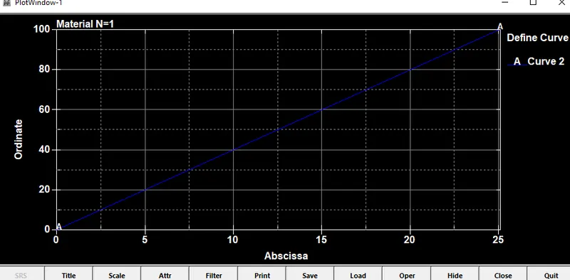
Open the Define_curve card and enter the values

Material Card

Enter

1. MID=1

2. RO= 0.0010

3. PR = 0.491

4. N= Number of constants to solve for = 1-3 for each case.

5. LCSS Load curve ID defining Engineering stress versus engineering strain LCID from Define_curve.

TENSILE TEST

The material is graphite iron casting for the meshed Dogbone specimen.

Boundary Conditions

For the tensile test, one end is fixed, one at centers, and the other end is given displacement. Hence 3 BCs.

1. Boundary_spc_set

• Constraint one end of the specimen in all directions except for Y because when it elongates in the X direction, the width along with Y contracts.
• Select the mid-nodes on both ends and constrain them for the Y direction.

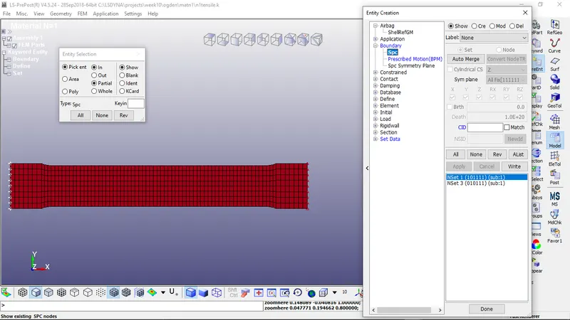
2. Boundary_Prescribed_Motion_set

A node_set is created at the other end of the specimen. In the tensile test, the strain should be at 100% so the displacement is given at 145mm, the same length as the specimen.

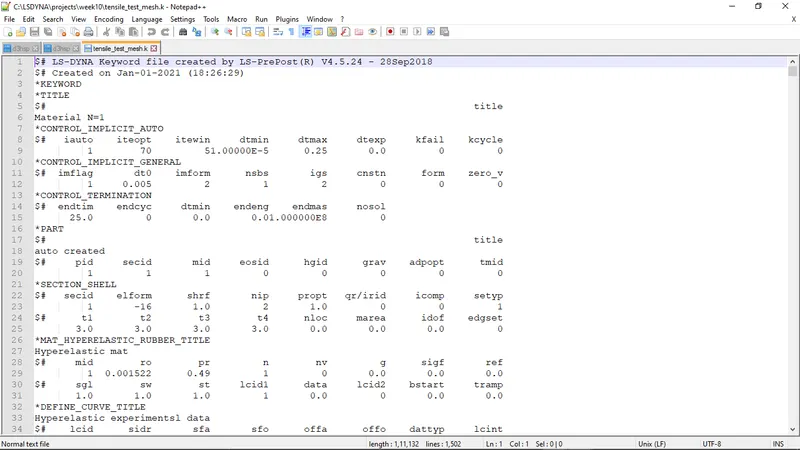
3. Control Implicit Auto parameters like general, solution, solver are set.

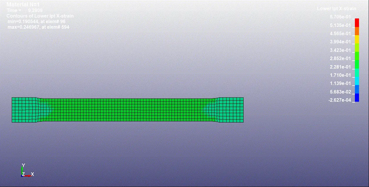
4. Database binary d3plot and ASCII cards- Glstat cards are created for knowing strain history.

5. The simulation with a given load curve is run and Mooney constants are obtained.

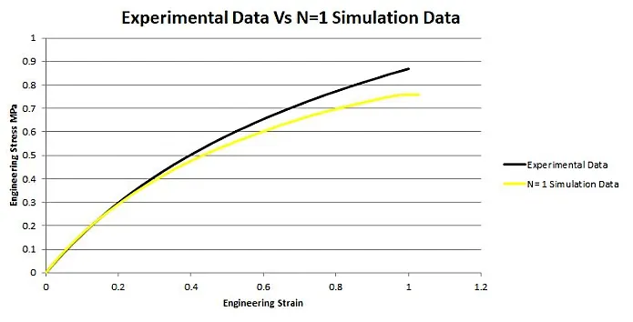
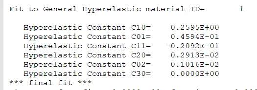
N=1

Mooney constant c1 = 0.1768E+00
Mooney constant c2 = 0.1474E+00

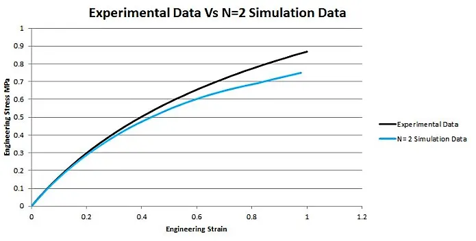
N=2

N=3

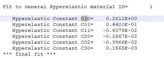
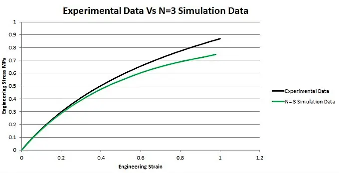
6. The fitted curve is verified and compared with given engineering stress and strain values.

7. The stretch is then converted to engineering strain (engineering strain= 1- stretch)

8. True stress is also converted to engineering stress. (engineering stress = True stress/(1+engg strain)

9. From the graph obtained, we can find that the fitted data curve follows the given data.

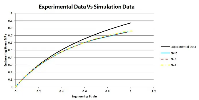
10. Taking the constants into consideration, the tensile test is simulated and validated.

11. The stress-strain data is plotted after simulation and the data is converted to engineering stress-strain values and plotted and compared with given data.

12. Using Ogden material, a similar process is carried out to validate the curve.

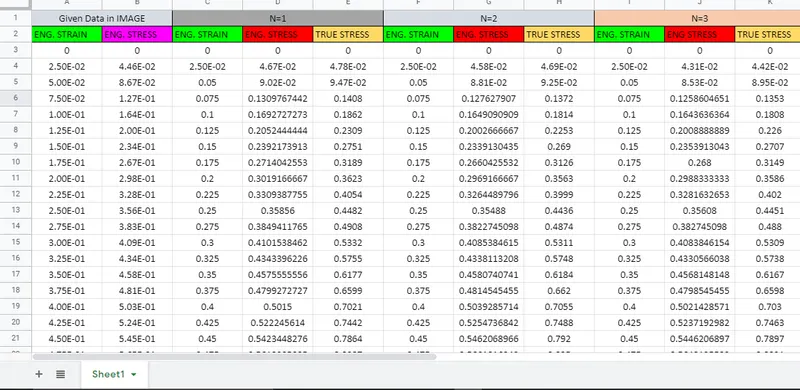
13. The graph is plotted and compared.

14. The constants are noted down and a tensile test is performed on the model to validate the derived constant.

15. The simulation data from the tensile test follows the data and is hence validated.

Model: https://drive.google.com/drive/folders/1TmFGw2tO0j4hYhaodWk9eho1STBl-kE8?usp=sharing

Conclusion

1. The hyperelastic material modeling is simulated for the tensile test with given load curve data.

2. The constants we obtained found out that the material curve is valid for the uniaxial stress data derived from the stress-strain element history curve.

3. The graph for n=1, n=2, n=3 is plotted and compared with experimental data.