Hyper-Elastic Material Modeling using LS-DYNA
Objective:
To perform the material modeling from the data given and calculate the Mooney Rivlin and Ogden material constants and compare the both using stress-strain data from a Dogbone specimen tensile test with 100% strain.
Hyper-elastic Material:
Hyperelastic material models are regularly used to represent the large deformation behavior of materials with FEA. They are commonly used to model mechanical behaviors of unfilled/filled elastomers. In addition to elastomers, hyperelastic material models are also used to approximate the material behavior of biological tissues, polymeric foams, etc.
Linearly elastic materials are described through two material constants (like Young’s modulus and Poisson ratio). In contrast, hyperelastic materials are described through a strain-energy density function. The strain-energy density can be used to derive a nonlinear constitutive model (i.e., stresses as a function of large strain deformation measures like deformation) which are derived by researches and some acceptable models we are using popularly such as Neo-Hookean, Mooney-Rivlin, and Signorini models, Ogden, Yeoh, Arruda-Boyce.
Mooney Rivlin Material Constant:
The strain energy density function for an incompressible Mooney–Rivlin material is defined as

Where; Cij">C_ij are empirically determined material constants, I1">I1and I2">I2 are the first and the second invariant. Similarly, we will be having multiple coefficients C. This changing of the index will be basically changing the order of the polynomial of the energy density equation. We need to find out the coefficients of these material models for a different order of the polynomial and extract the best fit curve data from the D3HSp file and compare it with the material curve.
Procedure
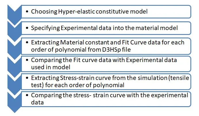
Hyper-Elastic Material Card:
As we are modeling a hyper-Elastic card, it is mandatory to use a material card that can access the necessary parameters pertaining to that of a hyperelastic material.
The following cards can be used to model a hyperelastic material,
*MAT_007 *MAT_BLATZ-KO_RUBBER- This is Material Type-7. This one parameter material allows the modeling of nearly incompressible continuum rubber. The Poisson’s ratio is fixed to 0.463.
*MAT_027 *MAT_MOONEY-RIVLIN_RUBBER-This is Material Type-27. A two-parametric material model for rubber can be defined.
*MAT_077_h *MAT_HYPERELASTIC_RUBBER This is Material Type-77. This material model provides a general hyperelastic rubber model combined optionally with linear viscoelasticity.
*MAT_077_o *MAT_OGDEN_RUBBER This is also Material Type-77. This material model provides the Ogden rubber model combined optionally with linear viscoelasticity.
Apart from these common hyperplastic materials for rubber there other material models too such as MAT_031, 038, 057, 063, 083, 092, 127, 129.
However, *MAT_007 is a very simple rubber model with just one parameter to defined i.e. (Shear Modulus) which cant be used for our case and *MAT_027 represents Mooney Rivlin constitutive model but this *MAT_27 will only solve with the First order of the polynomial.
So we will use *MAT_077_h which represents the Mooney Rivlin constitutive model and Different order of polynomial from 1 to 3 and find the Material constant for each order we can import a Load curve (experimental data value) and set SGL, SW, and ST parameters as 1 if the load curve is stress vs strain data.
Defining The Experimental data in the Material model:
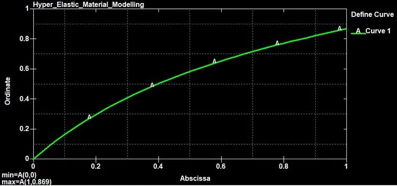
The stress/strain for the material is now in the form of Engineering stress and strain which can be directly implemented on the *MAT_77_h material card without any conversion.
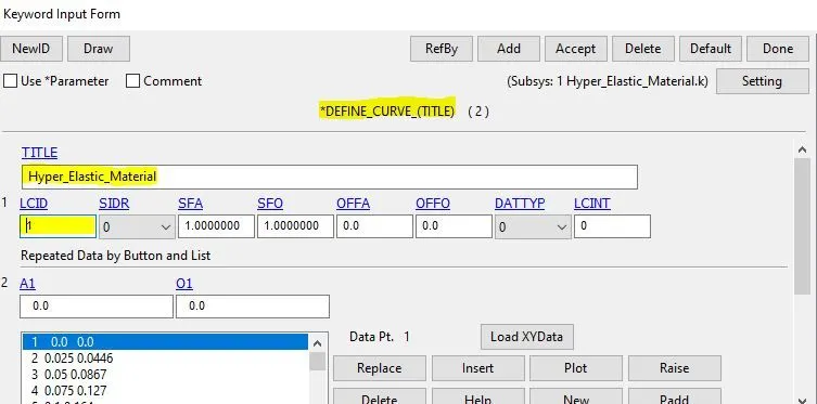
These data points for the Stress/Strain curve are inserted *DEFINE_CURVE Card with LCID.
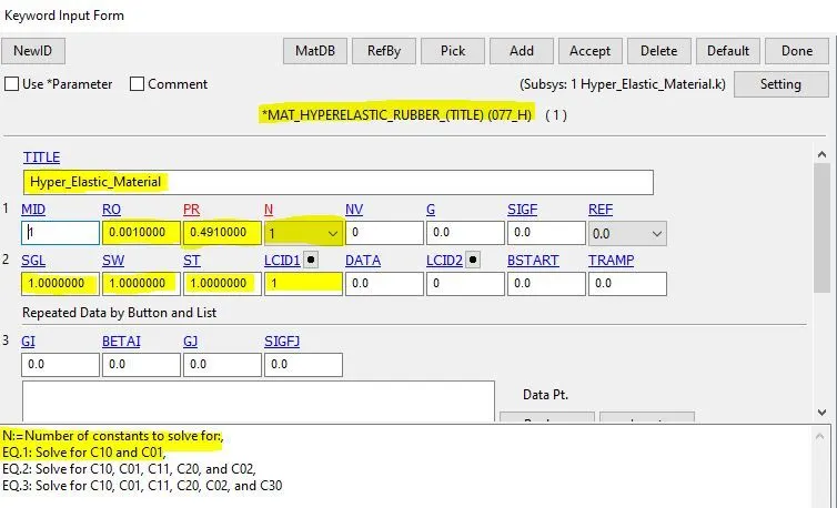
Material Card:
Then the next step is setting up the material card for the model. It is done through the command,
Model--->Keyword manager--->Mat--->*Mat_077_H_Hyperelastic_Rubber. Then the density, Poisson's ratio, and the curve is inserted into the model.
RO- Mass density= 0.00100
PR- Poisson’s ratio = 0.49100
N- Number of constants to solve for = 1-3 for each case
LCSS- Load curve ID defining Engineering stress versus Engineering strain LCID from *DEFINE_CURVE.
Boundary Condition:
Since we performing a Tensile Test where one end of the specimen is fixed and the displacement is added to the other end so we will use two types of boundary conditions on the Specimen.
BOUNDARY_SPC_SET:
To fix one end of the specimen as a test procedure we will constraint all the degrees of freedom except the Y direction (because the specimen will elongate in the X direction and simultaneously contract in Y) for the edge node on one end the specimen.
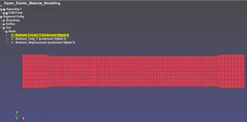
- We will select the mid-node on edge of both ends of the specimen and constrain only the Y direction
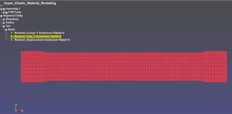
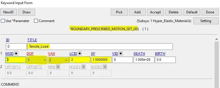
BOUNDARY_PRESCRIBED_MOTION_SET:
A set of nodes is created on the edge specimen in which displacement is applied.
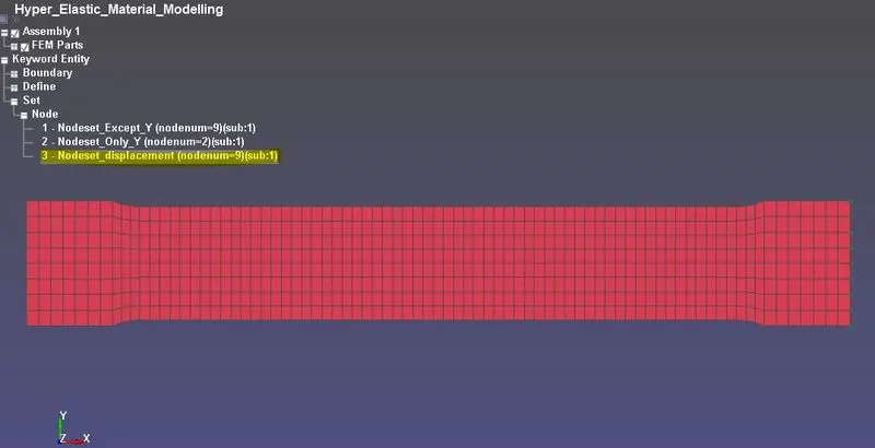
In the tensile test, the strain value as to be 100%. So we need to have the displacement the same as the length of the specimen. The specimen length is 145mm. So we need to have the displacement also like the 145mm. Displacement curve is created using Define_curve Card.
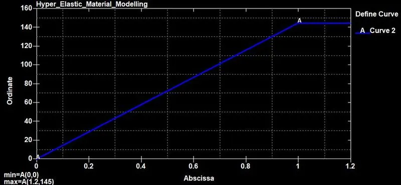
DOF in BOUNDARY_PRESCRIBED_MOTION_SET is set to be 1 which means displacement takes place in the X direction and VAD is set as 2 Displacement flag.
*CONTROL_IMPLICIT_GENERAL:
Activate Implicit analysis and define associated control parameters. This keyword is required for all Implicit analyses.
IMFLAG - Implicit/Explicit analysis type flag: 1- implicit analysis
DT0 – Initial time step size for implicit analysis: 0.0050000
IMFORM - Element formulation flag for seamless spring back: 2 retain original element formulation (default).
*CONTROL_IMPLICIT_SOLUTION:
Use of these cards to specify whether a linear or nonlinear solution is desired.
NSOLVER – Solution method for implicit analysis: 12 For Non-linear problem
ILIMIT-Iteration limit between automatic stiffness reformations: 11
MAXREF- Stiffness reformation limit per time step: 15
DCTOL- Displacement relative convergence tolerance: 001
DNORM- Displacement norm for convergence test: 2 (Increment as a function of total displacement)
*CONTROL_IMPLICIT_AUTO
This card has been defined to adjusts the time step size.
IAUTOset to 1 which automatically adjusts the timestep size.
ITEOPToptimizes the operation count step:20
ITEWINis the iteration window: 5
DTMIN Minimum allowable time step size: 1.0000e-05
DTMAXMaximum allowable time step size:0.2500
Database Creation:
*BINARY_D3PLOT - It defines the frequency at which the animation file is to be created and is set to 5.000e-05 ms.
*DATABASE_EXTEND_BINARY - this writes the strain tensor to d3plot when STRFLG is set to 1.
ASCII_option keyword
The output request in ASCII format, The following keyword are Activated
GLSTAT- Global Data,
MATSUM- Material Energies and,
ELOUT- Element Output Data.
Extracting Material constant and Fit Curve data for each order of polynomial from D3HSp file:
The Mooney-Rivlin constants for each case are stored in the d3hsp file.
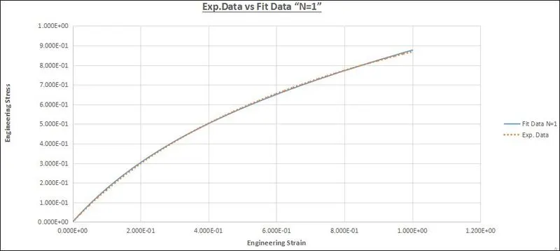
Case 1: N = 1 - First order polynomial;
- Mooney constant C01 = 0.1768E+00
- Mooney constant C10 = 0.1474E+00
Final Fit Data from the d3hsp file is generally in Stretch vs True Stress but We have to Covert them into Engineering Strain vs Engineering Stress
Engineering Strain = Stretch -1
Engineering Stress = True Stress/Stretch
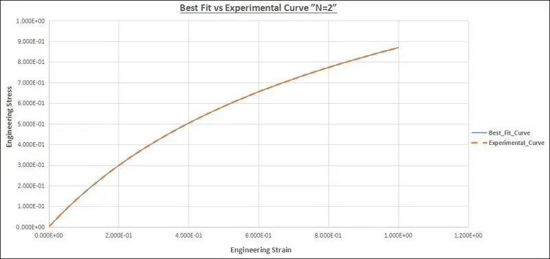
Case 2: N = 2 - Second order polynomial;
- Mooney constant C10 = 0.2595E+00
- Mooney constant C01 = 0.4594E-01
- Mooney constant C11 = -0.2092E-01
- Mooney constant C20 = 0.2914E-02
- Mooney constant C02 = 0.1016E-02
- Mooney Constant C30= 0.0000E+00
Case 3: N = 3 - Thrid order polynomial;
- Mooney constant C10 = 0.2611E+00
- Mooney constant C01 = 0.4420E-01
- Mooney constant C11 = -0.6074E-02
- Mooney constant C20 = -0.2667E-02
- Mooney constant C02 = -0.9968E-02
- Mooney constant C30 = 0.1565E-03
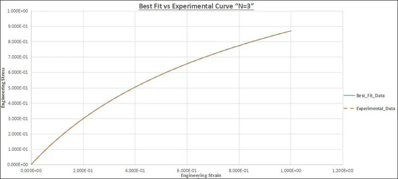
By Comparing, the 2nd & 3rd Order of polynomial, Final Fit data matches the Experimental data accurately compared to the 1st Order of polynomial. Now we will compare the Simulated Stress/Strain curve from the Tensile Test for Each order of the polynomial.
Comparison of Simulation Stress/Strain with Material experimental Stress/Strain data
Case 1: N = 1 - First-order polynomial;
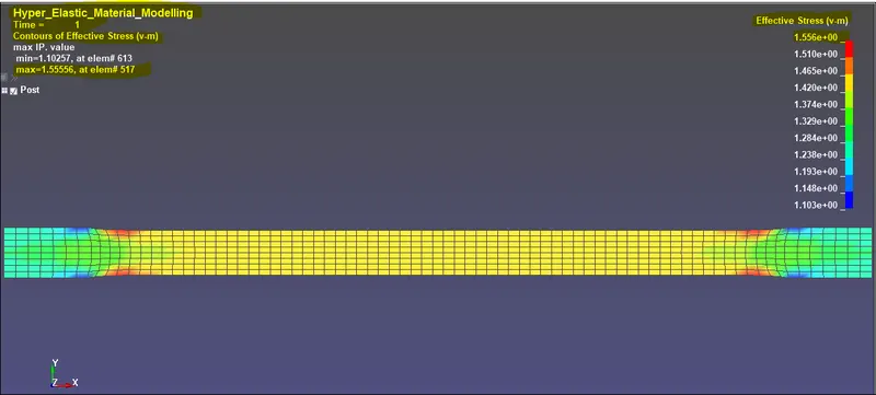
Effective Stress
Max Stress: 1.556MPa at Shell_Element-ID 517.
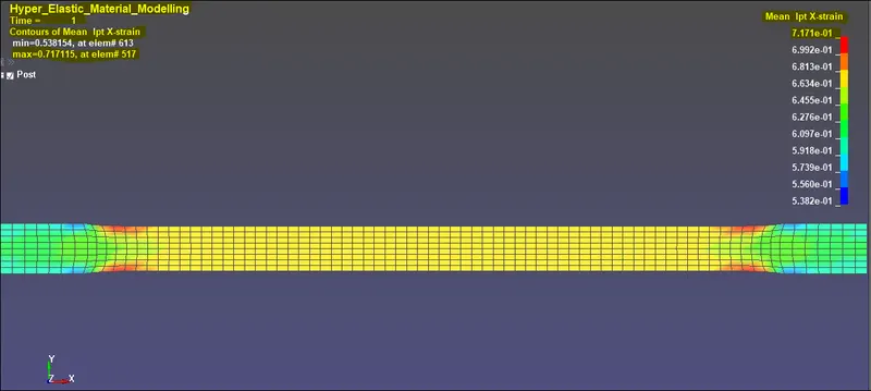
Mean Ipt X strain:
Max Strain: 0.717 at Shell_Element-ID 517.
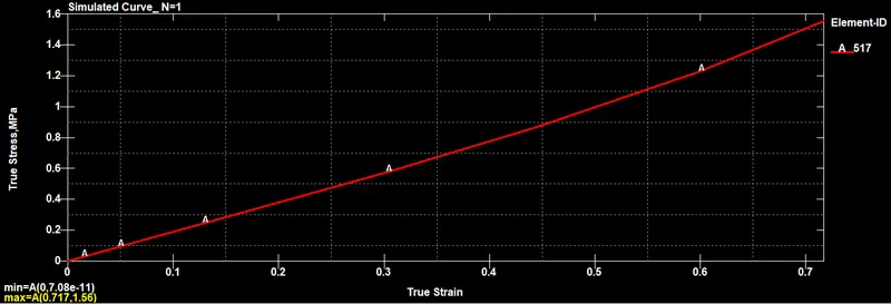
The stress and Strain curve is plotted for the element which is there in the mid-portion of the specimen.
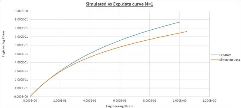
Since these are True stress Strain values we can convert them to Engineering Stress and Strain so that we can compare them with the Material experimental data.
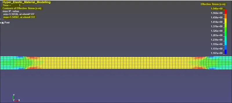
Case 2: N = 2 - Second-order polynomial;
Effective Stress:
Max Stress: 1.546MPa at Shell_Element-ID 517.
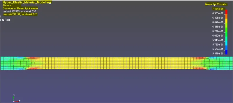
Mean Ipt X strain:
Max Strain: 0.716 at Shell_Element-ID 517.
Stress and Strain curve is plotted for the element which is there in the mid-portion of the specimen.
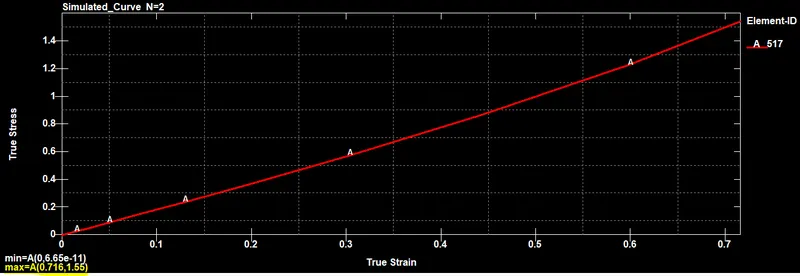
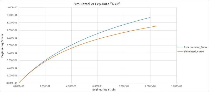
Since these are True stress Strain values we can convert it to Engineering Stress and Strain so that we can compare them with the Material experimental data.
Case 3: N = 3 - Third-order polynomial;
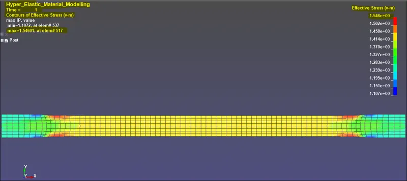
Effective Stress:
Max Stress: 1.546MPa at Shell_Element-ID 517.
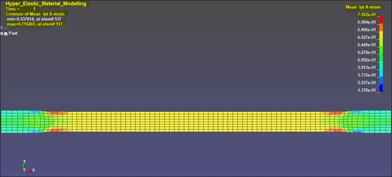
Mean Ipt X strain:
Max Strain: 0.7553 at Shell_Element-ID 517.
The stress and Strain curve is plotted for the element which is there in the mid-portion of the specimen.
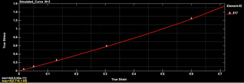
Since these are True stress Strain values we can convert them to Engineering Stress and Strain so that we can compare them with the Material experimental data.
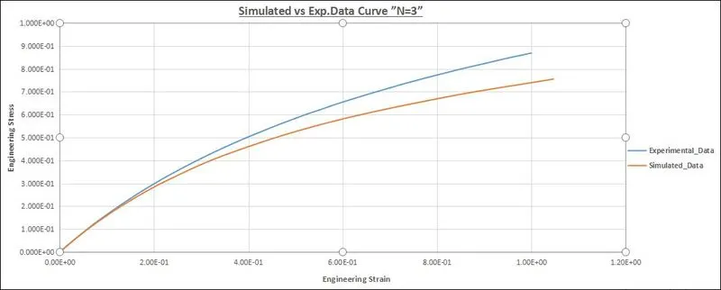
Observation for three cases:
As we can see the First Order Polynomial N=1 is closer to the Experimental data. So we can consider this as the best fit for our case and we can use the Mooney constant from First Order Polynomial N=1 in the Material Deck.
*MAT_077_o *MAT_OGDEN_RUBBER
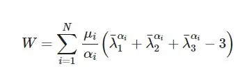
Ogden Hyper-elastic model is expressed the strain energy function W in terms of principal stretches, Where N is the order of the model, usually, N takes a number between 1–8. The same procedure is followed for building the Ogden Material Deck Since there 8 orders of polynomial in this material model we will use 1,2,3 order of polynomial for this case. Density, Passion ratio, SGL, SW, and ST parameters are set with the same value we used for MAT_077_h.
Extracting Material constant and Fit Curve data for each order of polynomial from D3HSp file:
The Ogden constants for each case are stored in the d3hsp file.
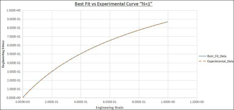
Case 1: N = 1-First order polynomial;
- mu_1= 0.9108
- alpha_1= 1.342
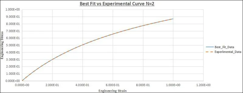
Case 2: N =2–Second order polynomial;
- mu_1= 9.156E-01
- mu_2= 2.225
- alpha1= 1.339
- alpha_2=-1.843E-03
Case 3: N =3–Third order polynomial;
- mu_1= -3.184E-02
- mu_2= 2.613E-01
- mu_3= 6.819E-01
- alpha_1= 1.926
- alpha_2= 1.550
- alpha_3= 1.289
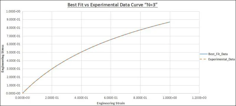
By Comparing, the 1st, 2nd, and 3rd Order of polynomial, Final Fit data they are very similar but they are very deviated from the Experimental data. so we will compare the Simulated Stress/Strain curve from the Tensile Test for Each order of the polynomial and check which Order of polynomial is better.
Comparison of Simulation Stress/Strain with Material experimental Stress/Strain data:
Case 1: N = 1 - First-order polynomial;
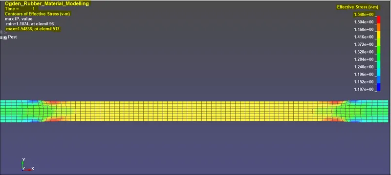
Effective Stress
Max Stress: 1.548MPa at Shell_Element-ID 517.
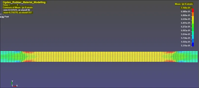
Mean Ipt X strain;
Max Strain: 0.717 at Shell_Element-ID 517.
Stress and Strain curve is plotted for the element which is there in the mid-portion of the specimen
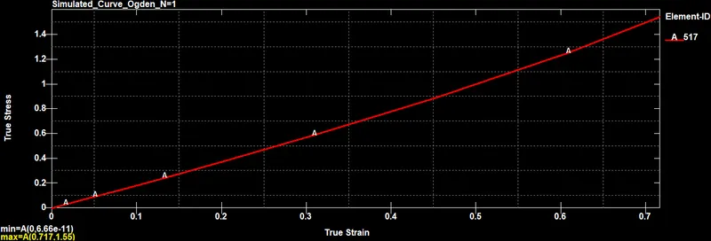
Since these are True stress Strain values we can convert them to Engineering Stress and Strain so that we can compare them with the Material experimental data.
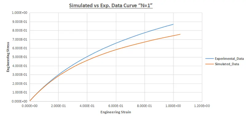
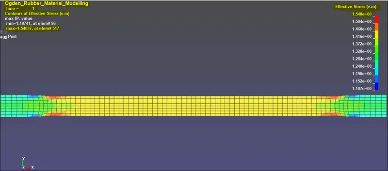
2. Case 2: N = 2-Second-order polynomial;
Effective Stress:
Max Stress: 1.548MPa at Shell_Element-ID 517.
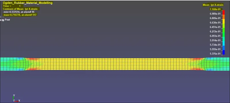
Mean Ipt X strain
Max Strain: 0.7170 at Shell_Element-ID 517.
The stress and Strain curve is plotted for the element which is there in the mid-portion of the specimen.
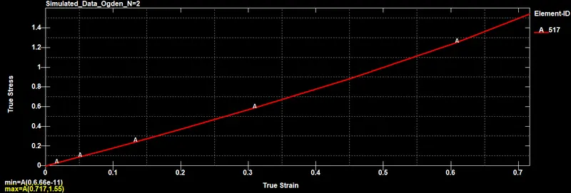
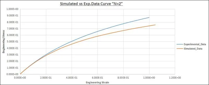
Since these are True stress Strain values we can to convert it to Engineering Stress and Strain so that we can compare with the Material experimental data.
Case 3: N = 3-Third-order polynomial;
Effective Stress:
Max Stress: 1.548MPa at Shell_Element-ID 517.
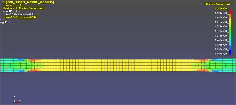
Mean Ipt X strain:
Max Strain: 0.7171 at Shell_Element-ID 517.
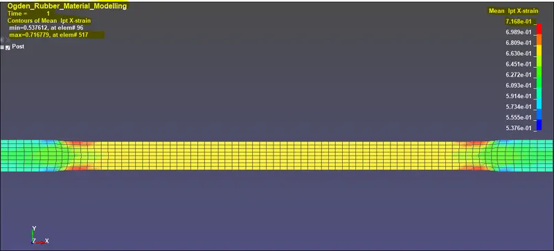
The stress and Strain curve is plotted for the element which is there in the mid-portion of the specimen.
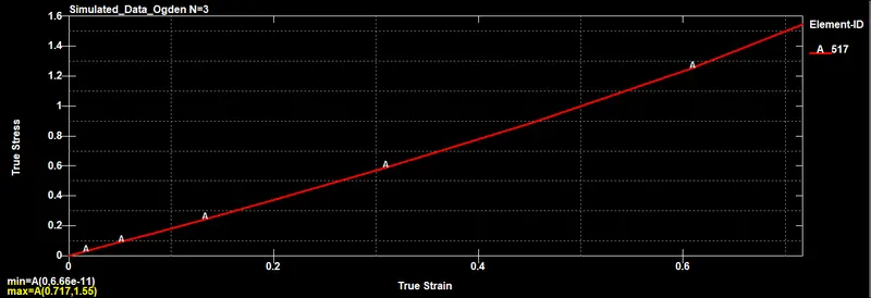
Since these are True stress Strain values we can convert them to Engineering Stress and Strain so that we can compare them with the Material experimental data.
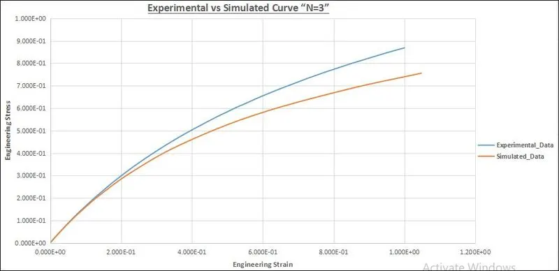
As we can see all the order of the polynomial looks same but if we look at the data points values more closer we can say N=3 is better than the other two order of the polynomial.
Conclusion:
We created two different hyperelastic material models and understood how each constitutive model works We extracted the material constant for Mooney–Rivlin and Odgen material for each order of the polynomial.
The solver tries to perform curve fitting for each order of polynomial with the actual material data And we compared which order tries to fit the material curve closer and as conclusion 2nd and 3rd order of polynomial have closer value with material data.
We perform the simulation and compare the simulation stress and strain curve with the actual material curve but the Simulation stress and Strain curve data depends on the material properties like (Poisson ratio and density) and since We have approximately defined these like Poisson ratio and density value so we can’t expect them to match the material curve exactly. After comparison, we can Say N=2 is better For Mooney–Rivlin Hyperelastic material.
The N=3 is better for Odgen Hyperelastic Material. Its because they fit the material original Stress and Strain curve closer than other order of the polynomial.