Week - 10 Hyperelastic Material Models
Objective : To model a hyper-elastic material card using the test data given and validate the results in the simulation.
Procedure :
Obtaining Stress-Strain data :
First we extract the engineering stress/strain data from the picture given and input it into an excel sheet.
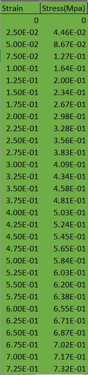
The data given is in engineering stress/strain. The unit system chosen is g,mm,ms.
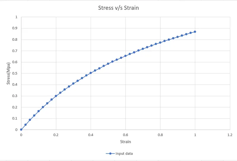
We will now plot the stress vs strain curve upto a strain of 1 which is upto where the data is provided.
Mooney-rivlin material card :
Creation of Material Card (Mooney Rivlin) :
Now we will create the material card. First we will input the data into LS-DYNA using Define-->Curve option.
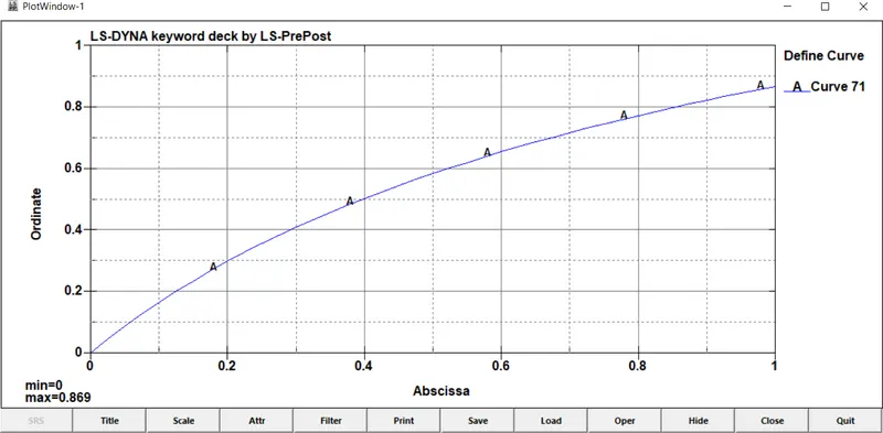
As the data is quite clear and strain values are taken at uniform intervals, we do not need to clean up the data and can directly input it.We create the load curve with ID 71.
Next we will create a new material card as such.
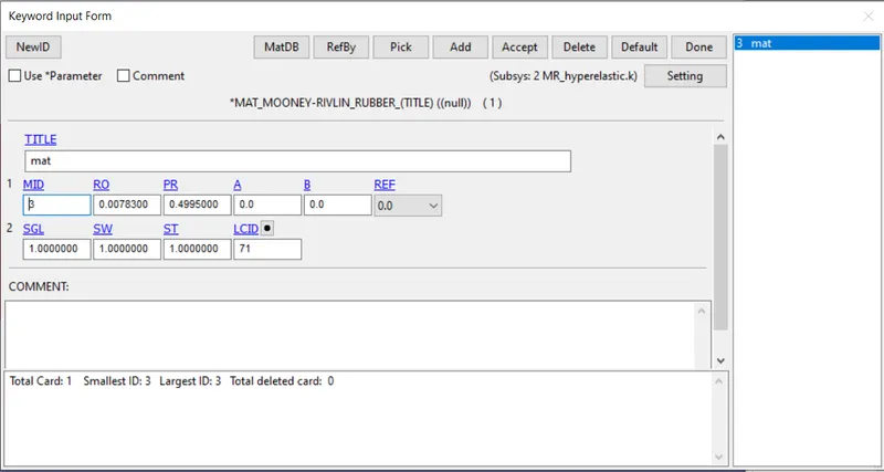
Enter the density, Poisson's ratio values and keeping SGL, SW, ST as 1 we can enter an engineering stress/strain curve into LCID.
Setting up the simulation :
Next we will set up the implicit simulation.
Boundary conditions :
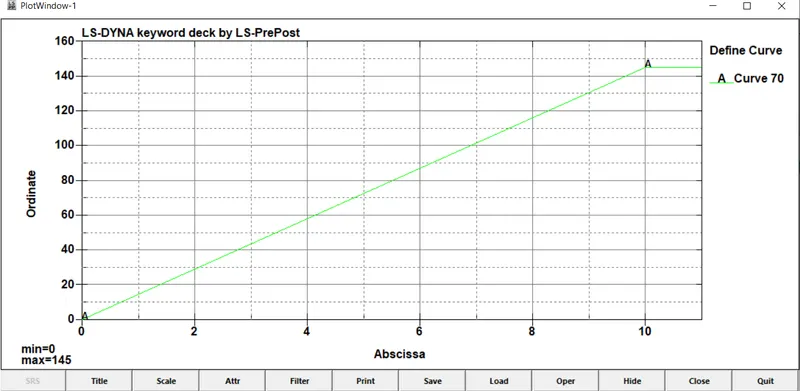
Prescribed motion is applied at one end of the dogbone specimen of the order of 145mm which makes the strain 100% as is given in the curve. The following displacement curve is used.
SPCs :
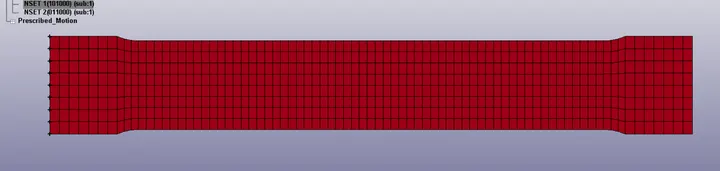
The nodes at the other end are restricted along x & z axes.
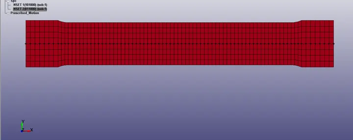
The nodes along the center line are restricted along y & z axes to constrain the neutral axis.
Creation of part :
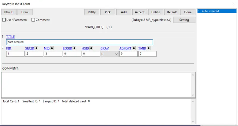
The section ID and material ID are assigned to the part.
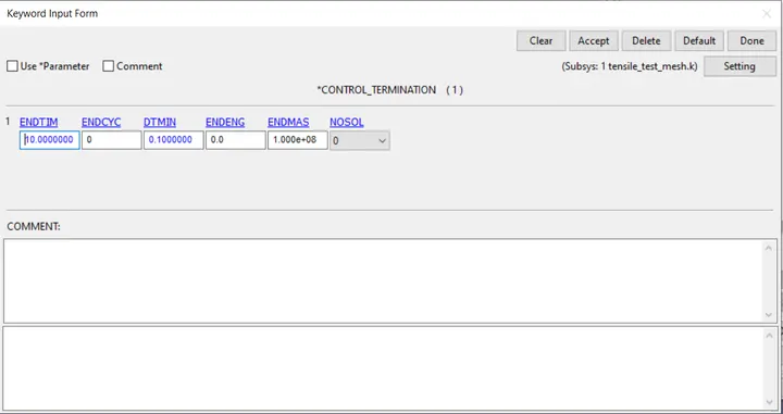
Control parameters :
The termination time is set at 10 ms.
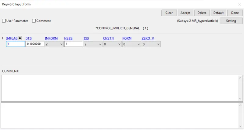
CONTROL_IMPLICIT_GENERAL
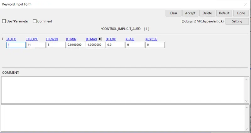
CONTROL_IMPLICIT_AUTO
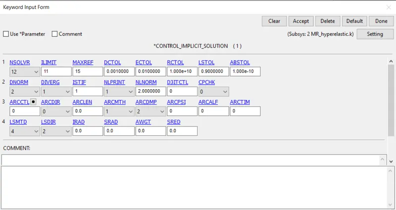
CONTROL_IMPLICIT_SOLUTION
Database options :
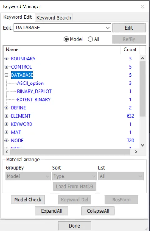
The following options are selected in the database for output of data.
Running the Simulation (Mooney-Rivlin):
Now we will run the simulation.
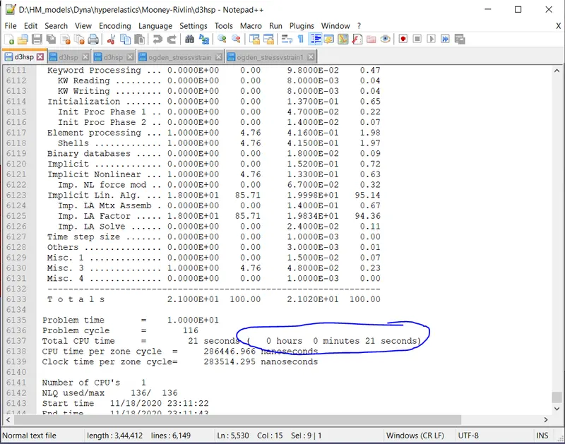
As we can see the simulation has a run-time of 21 seconds.
Comparison with input data :
We can obtain the stress/strain data after the initialization of the simulation from the d3hsp file.
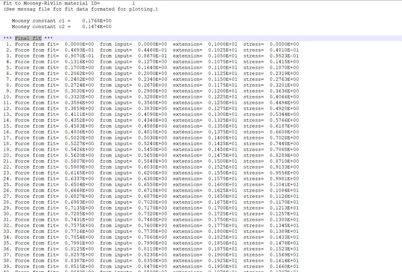
The constants c1 & c2 are noted down. We take the extension/stress data from this file and copy it to an excel sheet. To obtain strain from extension we subtract it by 1.
Also the stress value obtained here is true stress, we need to convert it to engineering stress to compare it with our input data.
We have the formula : Engineering stress = True stress/(1 + engineering strain)
Hence we obtain the engineering stress/strain values from this data.
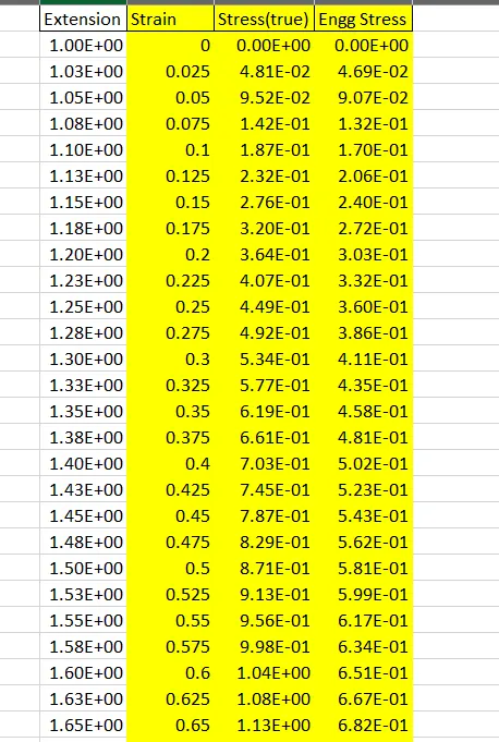
We then plot the data obtained from the simulation alongside the input data in a graph format like this to validate the results.
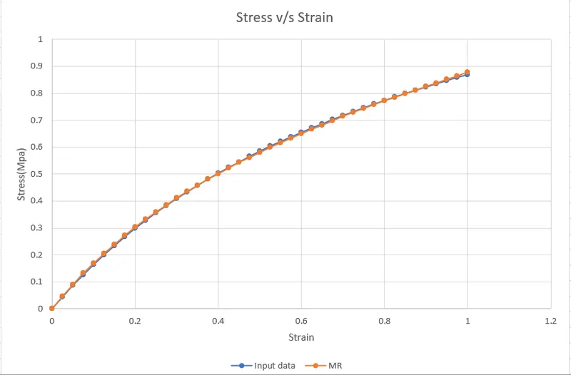
Hence we can see the data from the simulation matches correctly with our input data.
Comparison with constants input simulation :
In the above simulation we entered the material data using a load-curve. Now we will enter the material data using the constants that were generated during the simulation run and see if we get a matching result.
Creating material card :
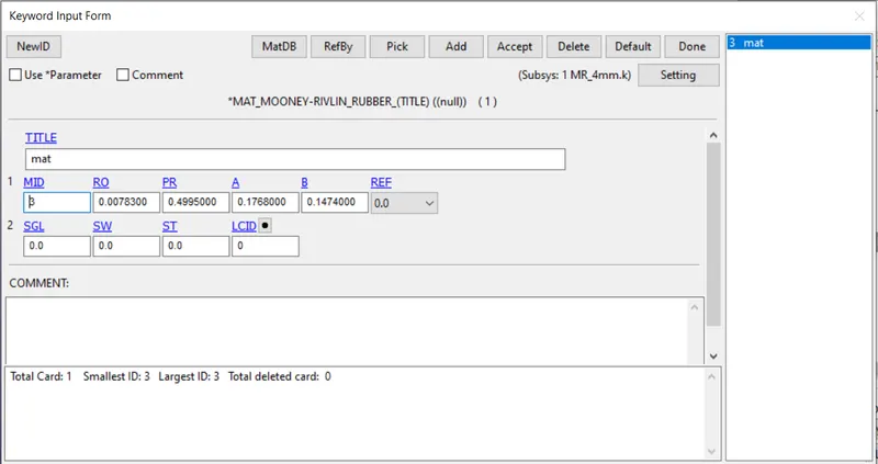
| Mooney constant c1 = 0.1768E+00 |
| Mooney constant c2 = 0.1474E+00 |
We will enter the above 2 values in the A & B column option instead of inputting the load curve as shown below.
Run the simulation :
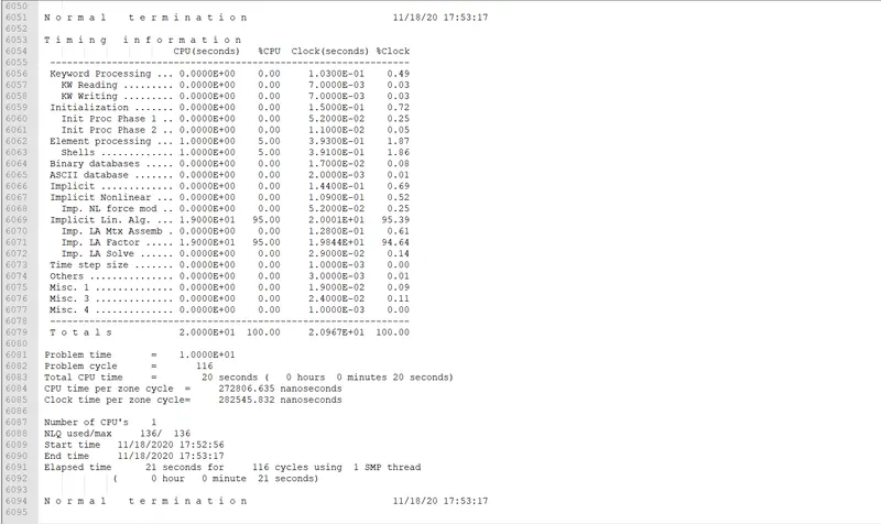
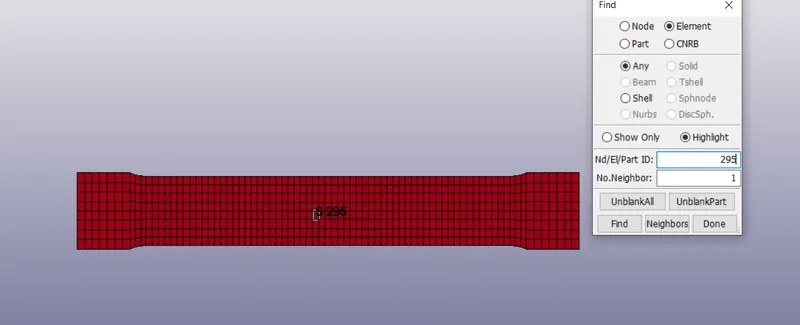
We see that the simulation now runs 1 second quicker and completes by 20 seconds as shown above. To compare the result the stress -strain curves are plotted for the element number 295 in both the cases. This element lies in the middle of the dog-bone specimen and will help us get a good result.
The stress -strain curve values are copied to an excel sheet and a graph is plotted as shown below.
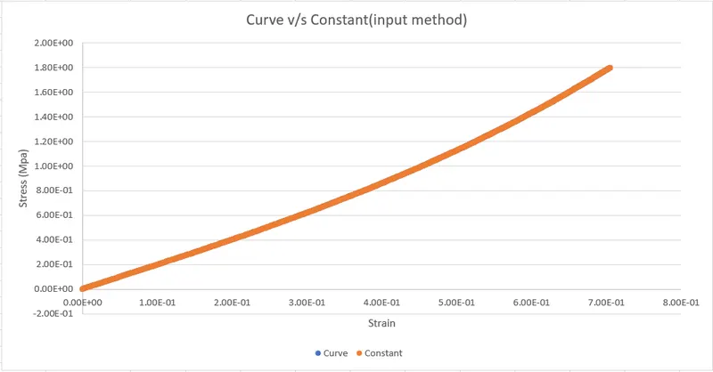
As we can see the reults is identical as the curve are overlapping one another. Hence we have concluded that by inputting the constants instead of load curves, we can obtain identical results at lowered computational time.
Ogden material card :
Creation of Material Card (Ogden) :
To create the Ogden material card create type 77 card as shown below, enter density, Poisson's ratio and N=8 to generate maximum number of constants so we can validate it better.
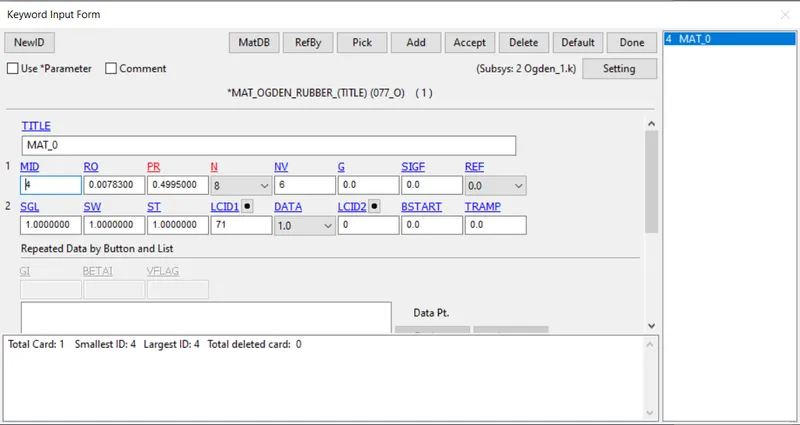
Enter SGL, SW, ST as 1 and enter the load curve. In Ogden material card we must define the strain for a greater value than what is supposed to run in the simulation. Hence to get a strain of 1 we must define the stress strain curve for a strain value more than 1.
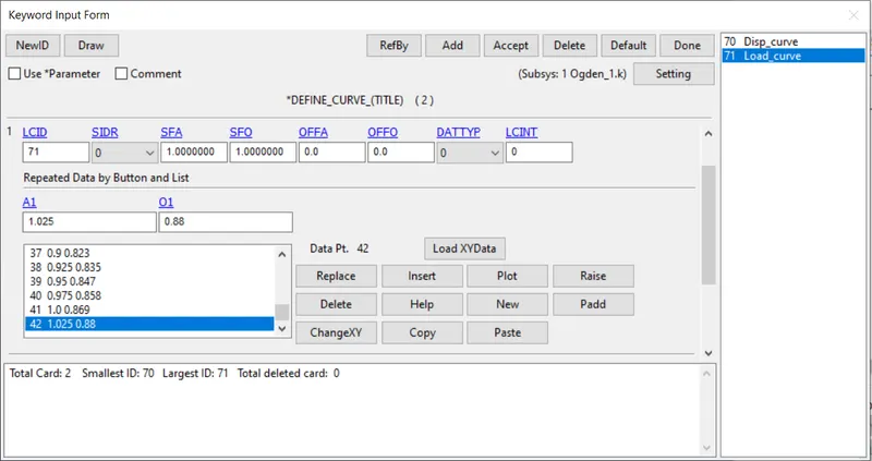
We will insert an additional point for strain of more than 1 looking at the previous point and provide an arbitrary stress value as shown above.
The rest of the simulation is exactly the same. So we will run it.
Running the Simulation (Ogden):
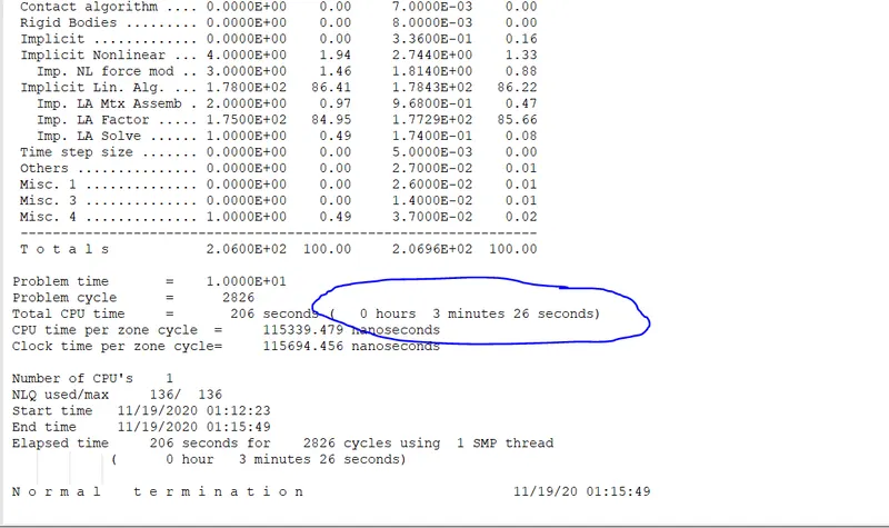
The simulation has a run-time of 3 minutes 26 seconds as shown above.
Comparison with input data :
We can obtain the stress/strain data after the initialization of the simulation from the d3hsp file.
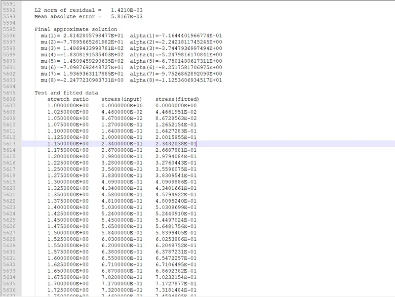
The constants
mu1,alpha1
mu2,alpha2
mu3,alpha3
mu4,alpha4,
mu5,alpha5,
mu6,alpha6,
mu7,alpha7,
mu8,alpha8
are noted down. We take the extension/stress data from this file and copy it to an excel sheet. To obtain strain from stretch ration we subtract it by 1.
The stress value obtained here is Engineering stress, so there is no need to convert it and we can directly compare it with the input data.
Hence we obtain the engineering stress/strain values from this data.
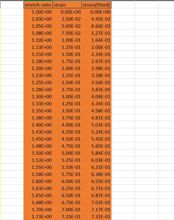
We then plot the data obtained from the simulation alongside the input data in a graph format like this to validate the results.
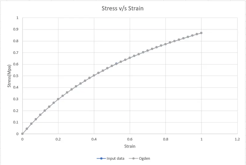
As we can see the data is more accurate and matches the input data more accurately when compared to Mooney-Rivlin method. Upto 2 decimal places the values match the input data exactly.
Comparison with constants input simulation :
In the above simulation we entered the material data using a load-curve. Now we will enter the material data using the constants that were generated during the simulation run and see if we get a matching result.
Creating material card :
| mu(1)= 2.8142805798477E+01 | alpha(1)=-7.1644401966774E-01 |
| mu(2)=-7.7895665261982E+01 | alpha(2)=-2.2421811745245E+00 |
| mu(3)= 1.4869433998781E+02 | alpha(3)=-3.7447936997494E+00 |
| mu(4)=-1.8308191535403E+02 | alpha(4)=-5.2479816170841E+00 |
| mu(5)= 1.4509459290635E+02 | alpha(5)=-6.7501480617311E+00 |
| mu(6)=-7.0987692448727E+01 | alpha(6)=-8.2517581706975E+00 |
| mu(7)= 1.9369363117885E+01 | alpha(7)=-9.7526862892090E+00 |
| mu(8)=-2.2477230983731E+00 | alpha(8)=-1.1253606934517E+01 |
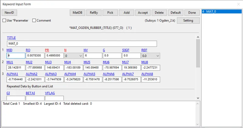
We will enter the above 8 values in the mu and alpha columns instead of inputting the load curve as shown below.
Keep N = 0 to get constants input mode in the material card.
Run the simulation :
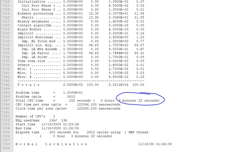
We see that the simulation now runs 4 second quicker and completes by 3 minutes & 22 seconds as shown above.
To compare the result the stress -strain curves are plotted for the element number 295 in both the cases. This element lies in the middle of the dog-bone specimen and will help us get a good result.
The stress -strain curve values are copied to an excel sheet and a graph is plotted as shown below.
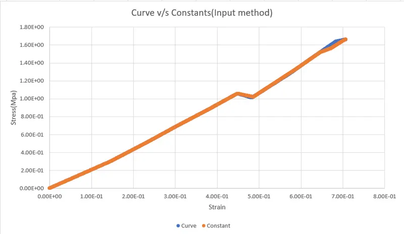
As we can see the reults is almost identical as the curve are overlapping one another. Hence we have concluded that by inputting the constants instead of load curves, we can obtain identical results at lowered computational time.
Comparison of 2 Material cards :
Finally we will compare the input data to the data obtained by the fit from both the material cards to obtain the following graph below.
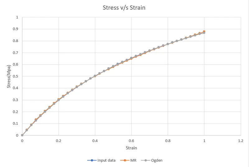
As we can see both the material models sufficiently represent the input test data with the Ogden model being slightly more accurate.
Conclusion :
Hence we have studied both the material cards to validate that the simulation is performing exactly like the test input data. We arrive at 2 conclusions :
- The Ogden material model is slightly more accurate than Mooney-Rivlin material card but is computationally more expensive.
- Hyper-elastic material cards can be defined using Constants or Load Curves to get identical results. However entering constants proves to be computationally less expensive.
Result :
Contents
1. Excel workbook containing 3 pages, one comparing the 2 material cards with test data and the other two comparing the simulations results of the individual cards using Load curve as input and Constants as input.
2. .K files of the simulations. (_1 for curve input, _2 for constant input)