Week - 10 Hyperelastic Material Models
Objective: Using the given material data, calculate the Mooney Rivlin and Ogden material constants and compare the both using stress-strain data from a Dogbone specimen tensile test with 100 percent strain. And analyze the comparison.
Brief Theory- Hyperelastic materials are the type of materials that has the potential of taking up to 500% strain and come back to the original state. It is a nonlinear but elastic material, material behavior is described in terms of strain energy as a function of stretch. Some examples- rubber, foam, adhesive.These models account for both nonlinear material behavior and large shape changes.Some models that are being used are Mooney -Rivlin, Neo -Hookean etc.Here we discuss modelling of Mooney -Rivlin and ogden material using the given stress strain data.
We are to calculate the coefficients of the material models used for different order of polynomial and The comparison from the d3hsp file and material curve is to be done.
We use the material card M077 Hyperelastic rubber material and then vary the N values to calculate the required coefficients.
Procedure:
1. The Engineering stress- Engineering strain data was extracted from the pic provided.
2. The data was input using the DEFINE curve option so that it could be feed to the material card.
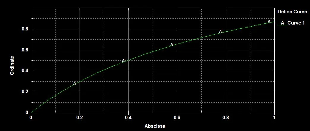 Fig: Curve for the material card
3. MAT077
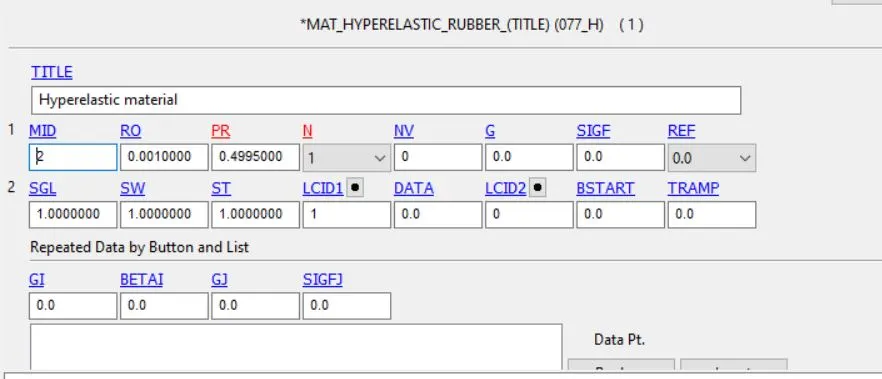
.Fig: Material card
4. The dogbone speciemen was included in order to proceed with the tensile simluation.
5.
Now, as we have to do a tensile simulation. Proper boundary condition has to be implemented.
1. We used SPC set, in one edge so that that end is fixed, (to compare with the sample being gripped), and keep it non constrained only in y translational direction (direction perpendular to the displacement provided in th expt)
2. Also the mid node on the two opposide edges are constrained in only the y translational and rotation about all axis.
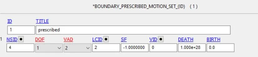
3. A prescibed boundary motion is applied on the opposite edge of the gripped boundary, and a displacement curve is defined.
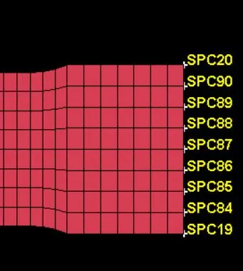
Fig : SPC on one edge
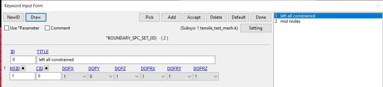
Fig : SPC on one edge card
 Fig:boundary spc mid node model
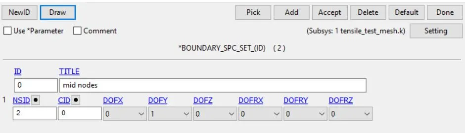
Fig:boundary spc mid node card
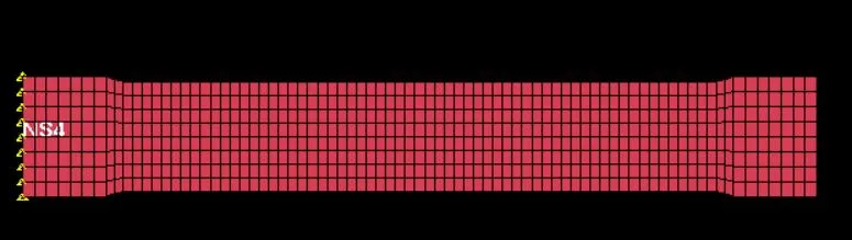
Fig: Prescribed nodes
Since it is mentioned Dogbone specimen tensile test with 100 percent strain, and as the length of the speciemen was 45 mm so the displacement curve as shown below to 145 mm.
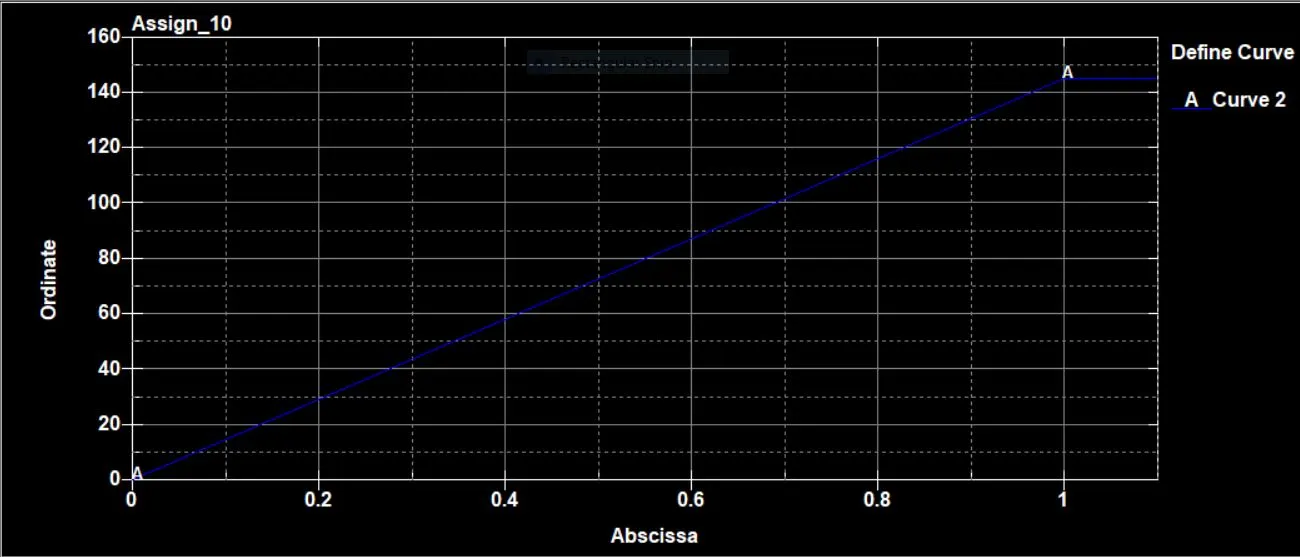 Fig: Displacement curve
Database History shell with element shell ID 314 was selected to get the strain data.
Since we need to extract stress-strain data, we need to define Extend database STRFLG =1,
As it is a quasistatic process we need to do implicit run, so control implict_General, Control_Implicit_auto is activated,
IAUTO= 1, and IMFLAG= 1.
The simulation was run.
For the case when N=1, the Mooney constants were extracted from the d3hsp file, also the curve fit in is in the outtput in the same file that is also extracted in excel and the output is in the form of extension and true stress, so it is converted to engineering strain and engineering stress by the below-mentioned formula.

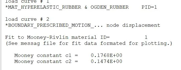
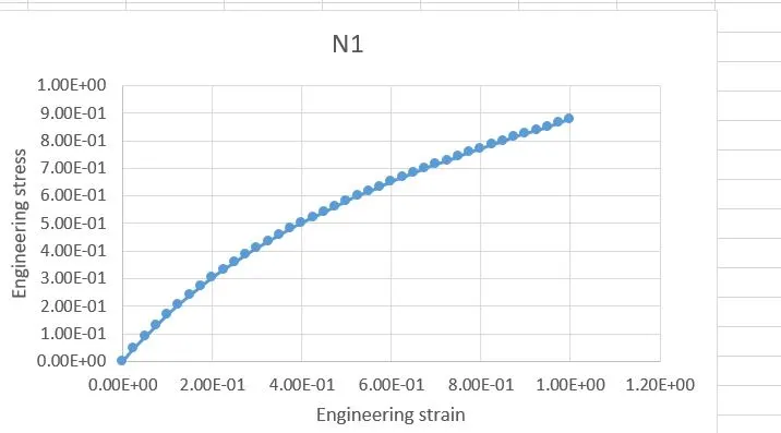
Fig: N1 :Eng. strain vs eng. stress extracted from d3hsp
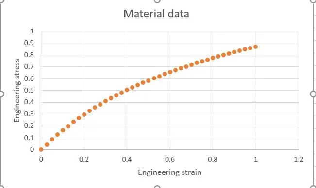
Fig: The engineering stress strain curve from the material data provided.
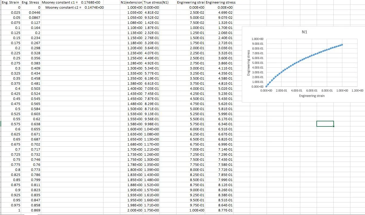
Now, the same simulation was run with N=2 , in the material card.
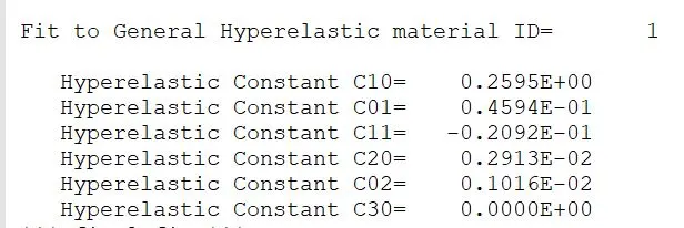
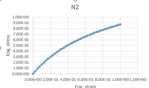
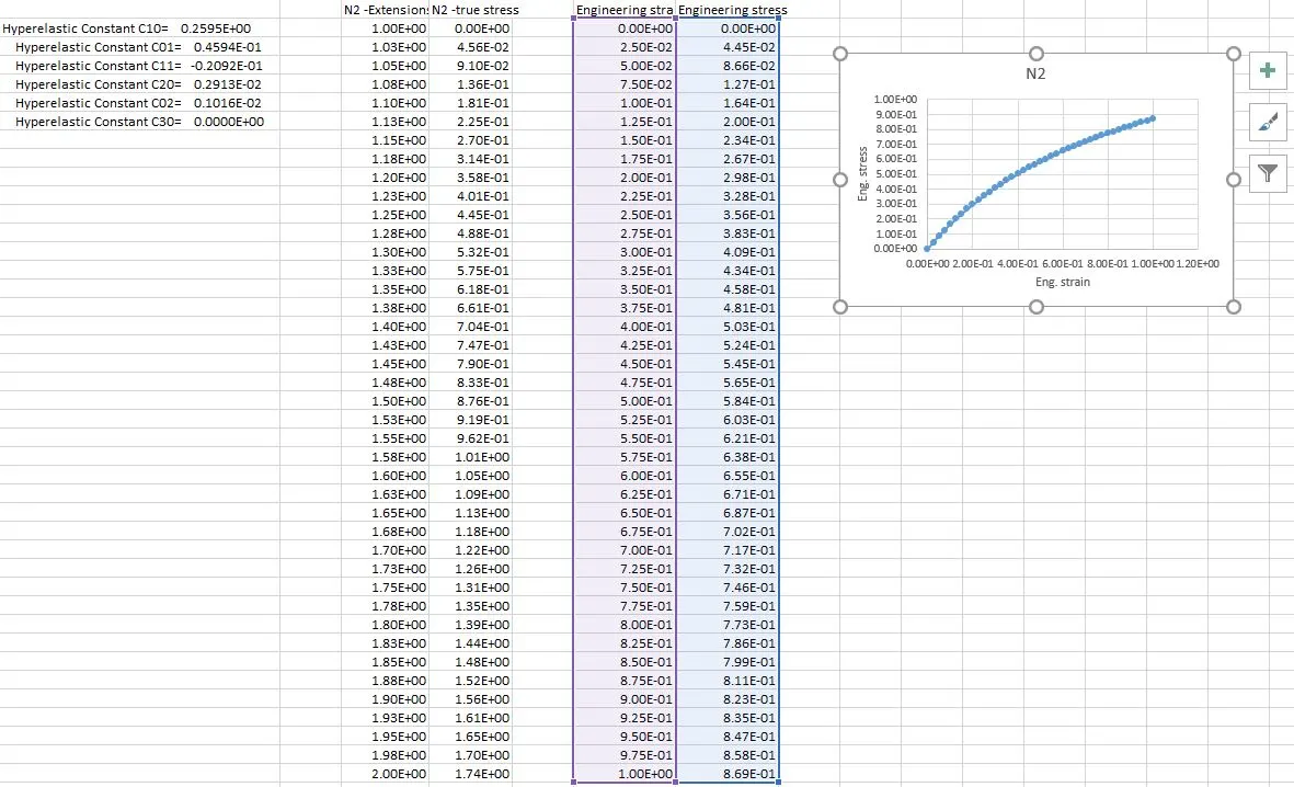
Now, the same simulation was run with N=3 , in the material card.
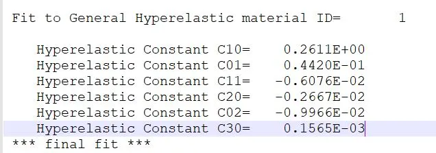
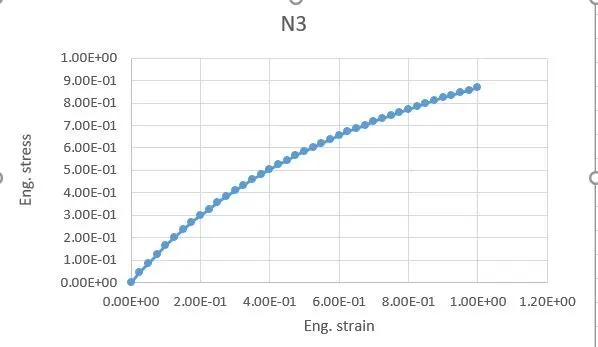
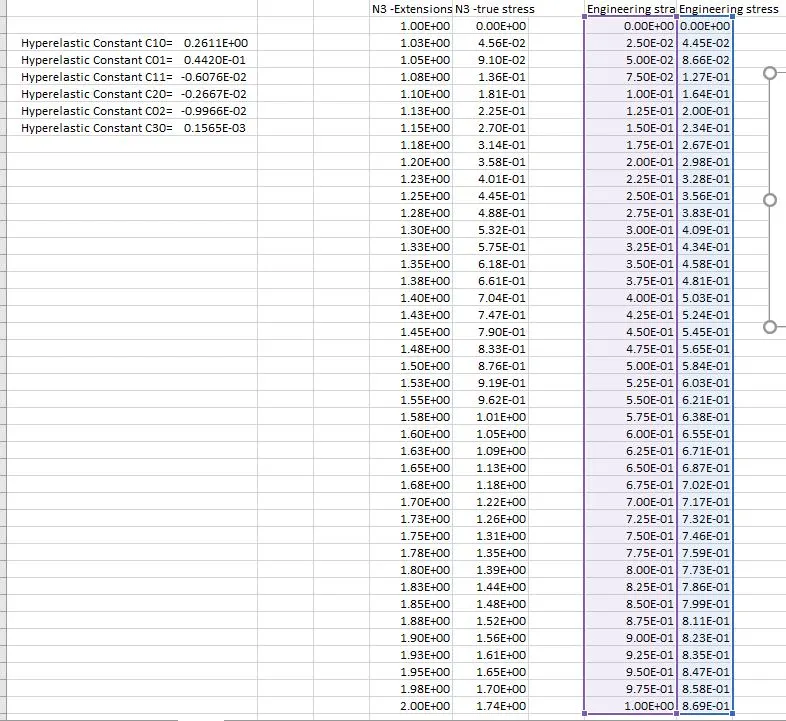
Now, uptill now, we can see that the stress-strain curve for N1, N2, and N3 and pretty similar.
Now , in order to validate the data, the constant set for each N simulations are fed into the material card by putting N=0 and the same simulation is run, and the result is analyzed, and then we can see that by using the history element we plot the lower ipt x strain and effective stress and this data is actually true strain and true stress, these are then converted to engineering stress and engineering strain and then plotted in order to compare with the material data provided in the question.
So, as mentioned first we study the case where, in the material card N =0 is assigned and then the constants for the first case by inputing the values of the constants C10 and C01.
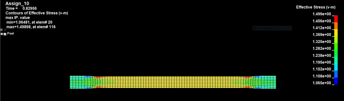
Fig: effective stress validation contour, the maximum and minimum effective stress are shown.
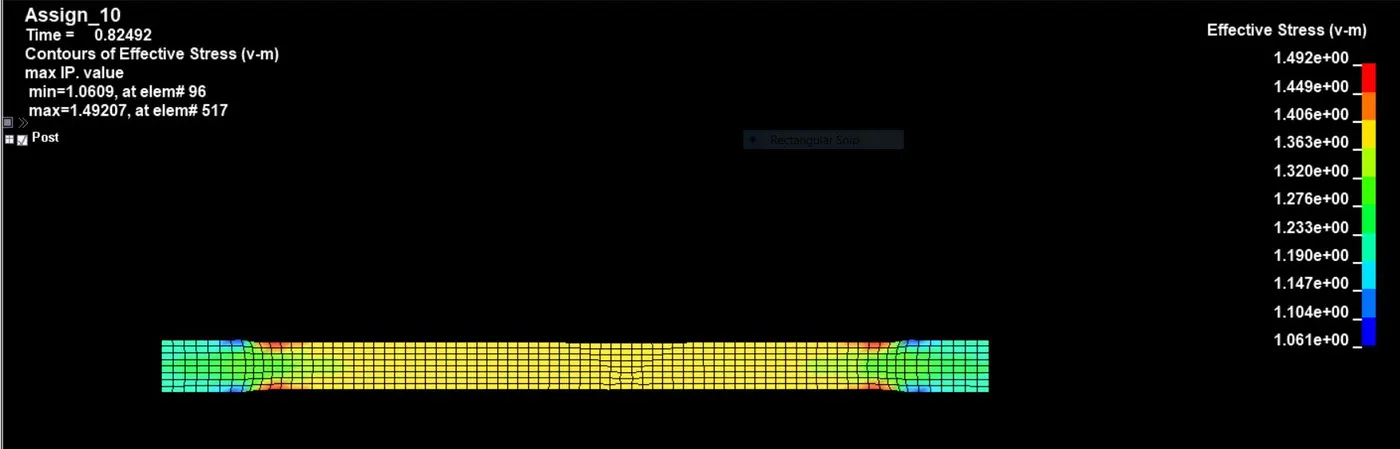
Fig: Effective stress contour (for the case where N1 is used), the maximum and minimum effective stress are shown.
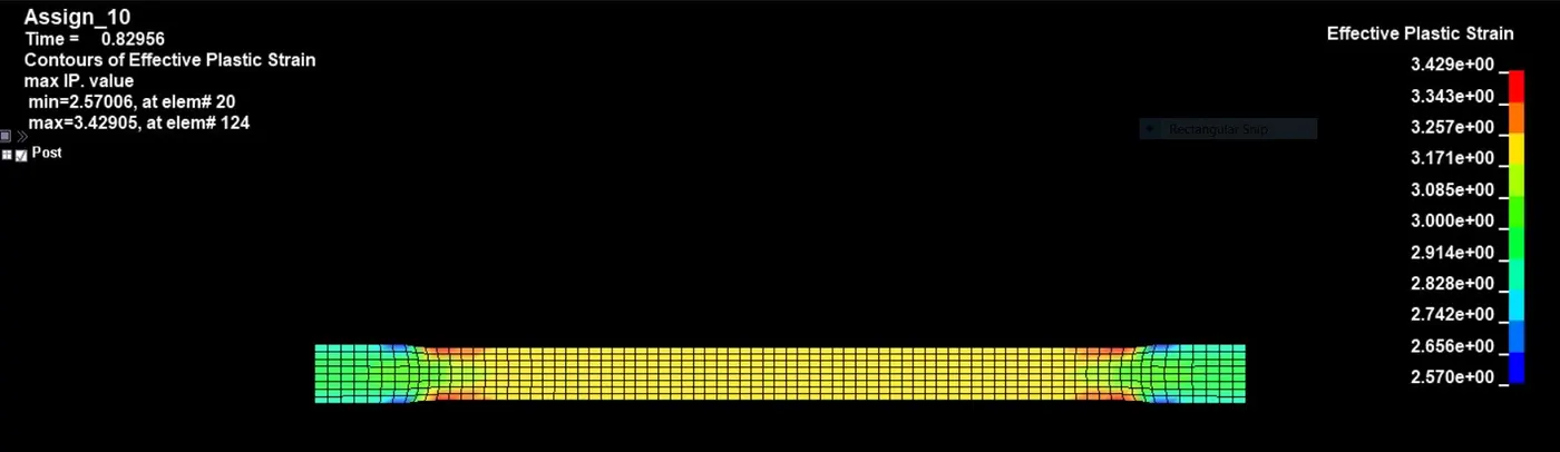 Fig: effective strain validation contour, the maximum and minimum effective stress are shown.
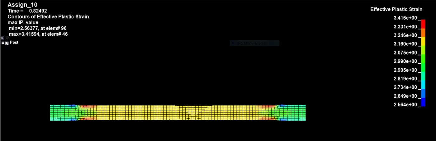 Fig: Effective strain contour (for this case where N1 is used), the maximum and minimum effective stress are shown.
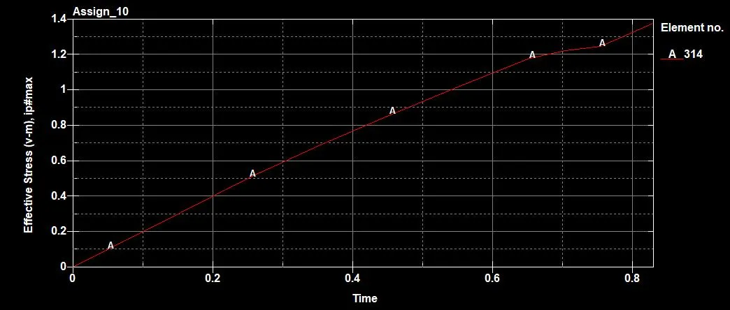 Fig: effective stress vs time (Validation case)
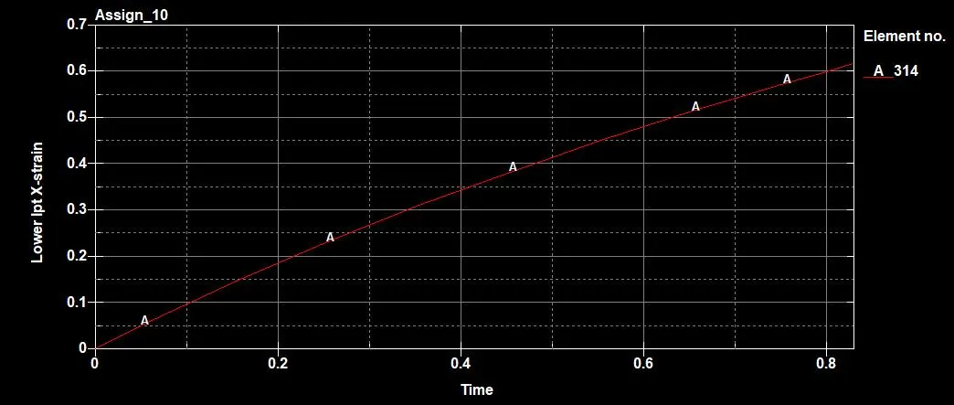 Fig: lower ipt x strain vs time (Validation case)
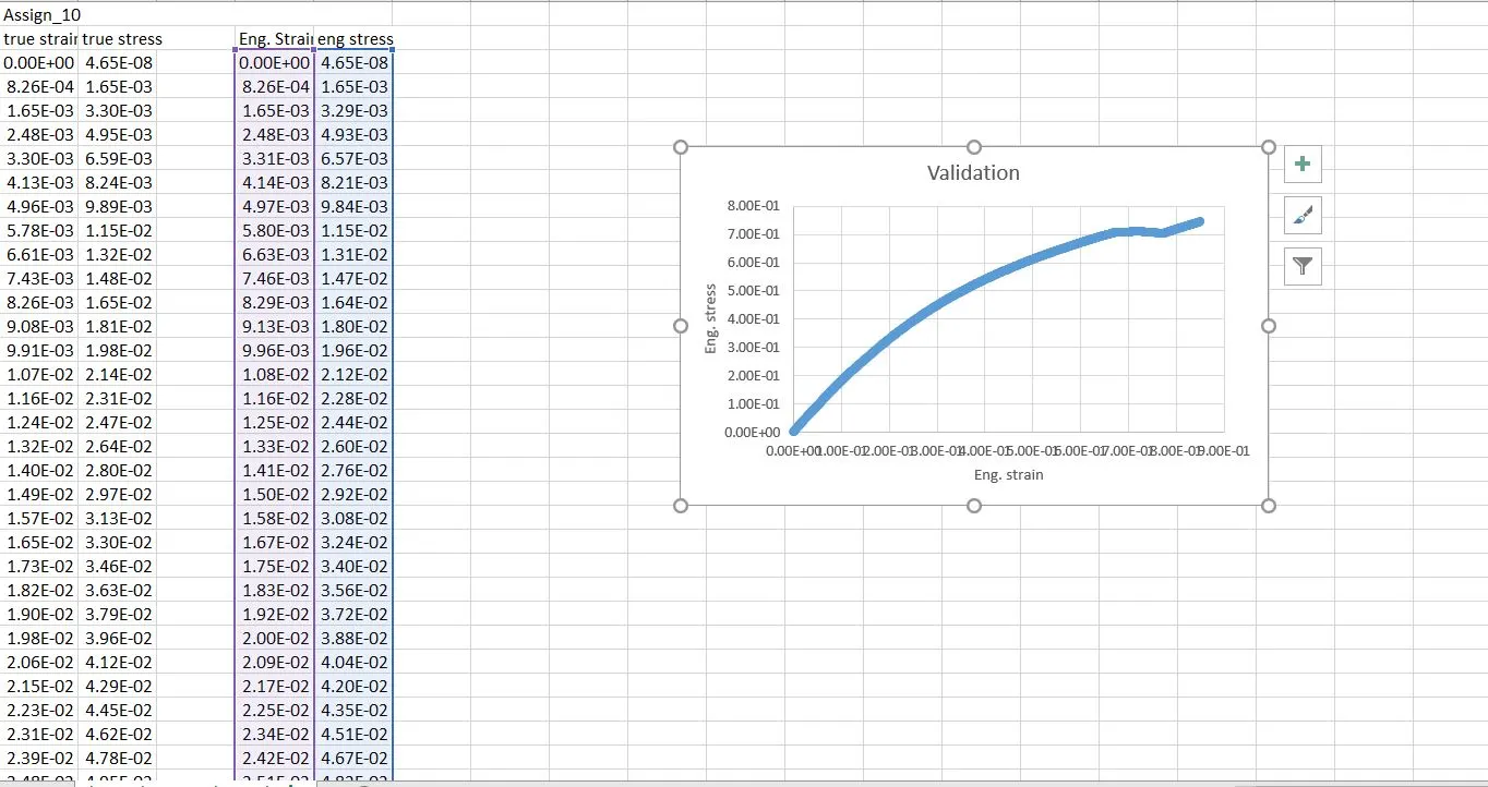
Fig: snapshot of excel sheet showing the calculation of each case where true stress - strain are converted to eng. stress- strain and the data is compared with the provided material data.
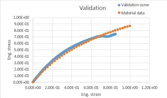
Fig : Comparision of the material data and validation
S0, as mentioned earlier, now we study the case where, in the material card N =0 is assigned and then the constants for the second case by inputing the values of the constants C10, C01, C11, C20.
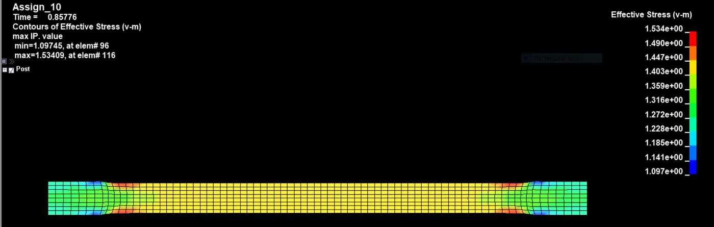
Fig: effective stress validation contour, the maximum and minimum effective stress are shown.
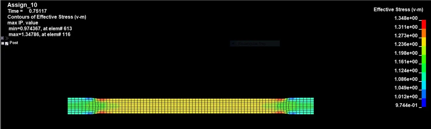
Fig: Effective stress contour (for the case where N1 is used), the maximum and minimum effective stress are shown.
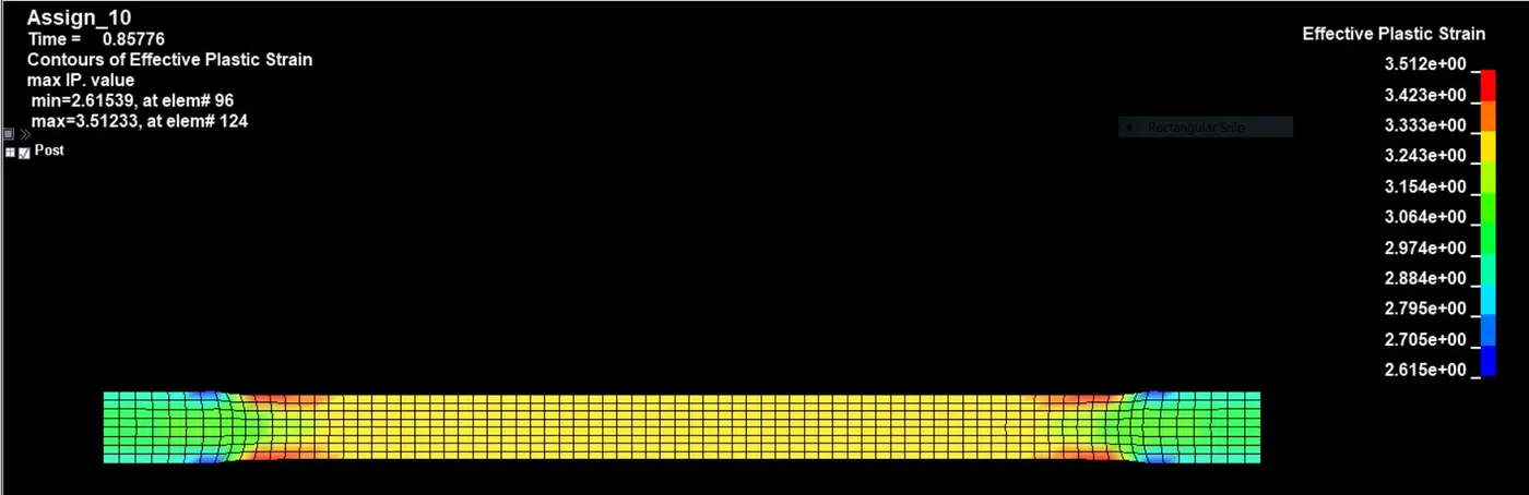
Fig: effective strain validation contour, the maximum and minimum effective stress are shown.
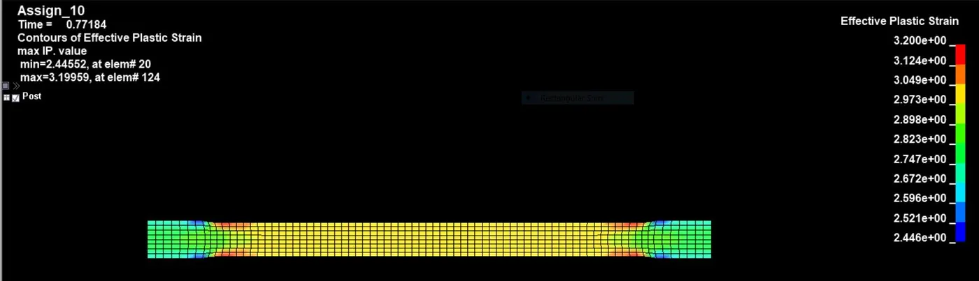
Fig: Effective strain contour (for this case where N1 is used), the maximum and minimum effective stress are shown.
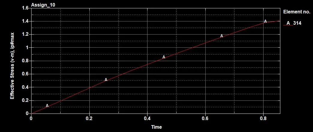
Fig: effective stress vs time (Validation case)
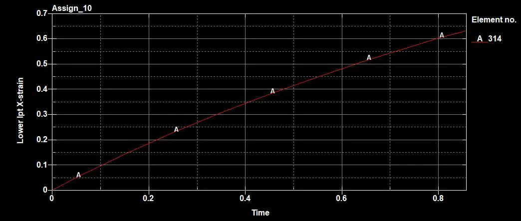 Fig: lower ipt x strain vs time (Validation case)
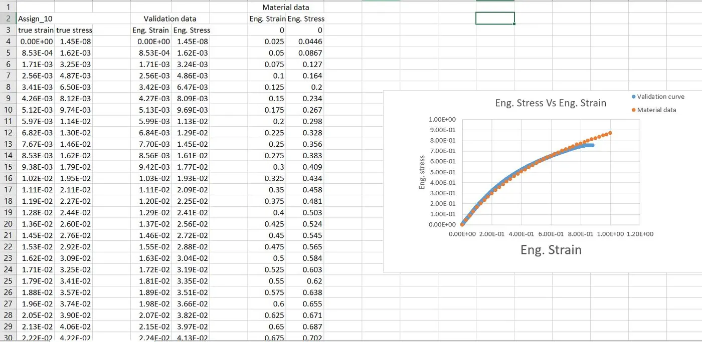
Fig: snapshot of excel sheet showing the calculation of each case where true stress - strain are converted to eng. stress- strain and the data is compared with the provided material data.
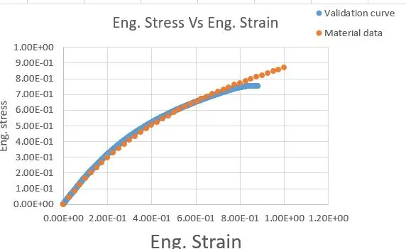
Fig : Comparision of the material data and validation
now we study the case where, in the material card N =0 is assigned and then the constants for the second case by inputing the values of the constants C10, C01, C11, C20, C02, C30
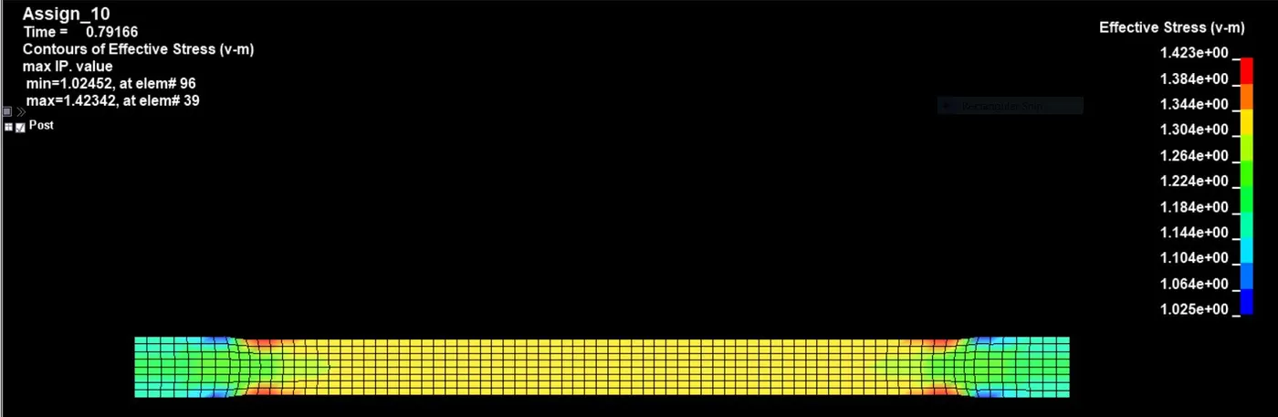
Fig: effective stress validation contour, the maximum and minimum effective stress are shown.
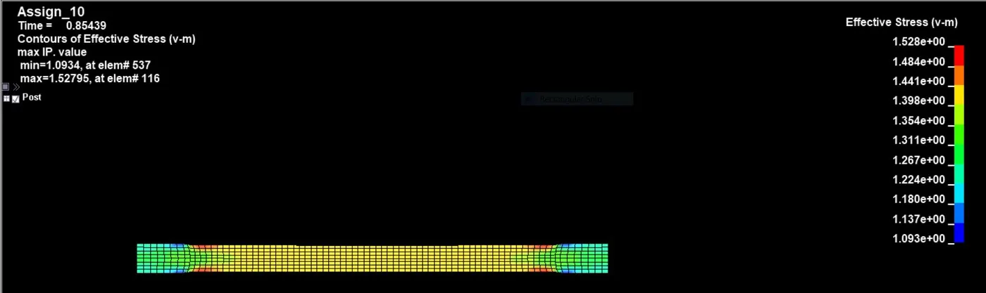
Fig: Effective stress contour (for the case where N1 is used), the maximum and minimum effective stress are shown.
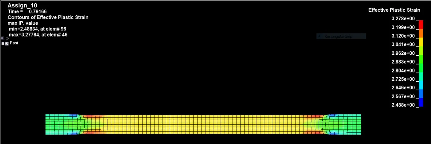
Fig: effective strain validation contour, the maximum and minimum effective stress are shown.
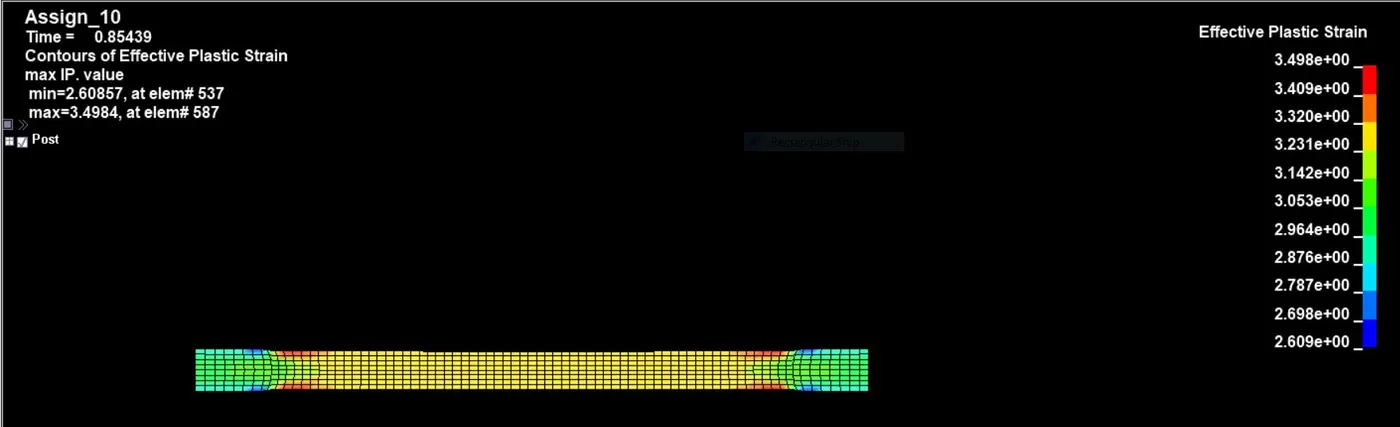
Fig: Effective strain contour (for this case where N1 is used), the maximum and minimum effective stress are shown.
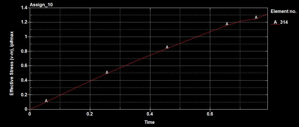
Fig: effective stress vs time (Validation case)
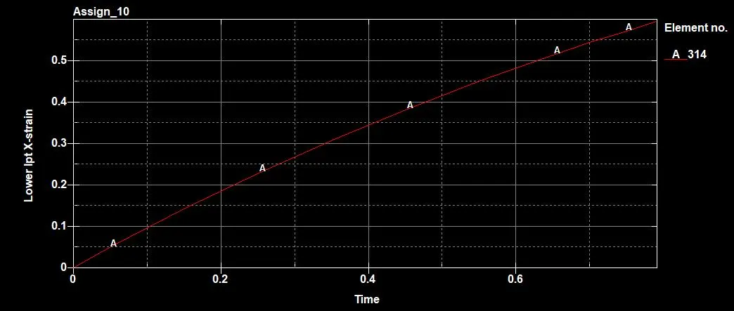
Fig: lower ipt x strain vs time (Validation case)
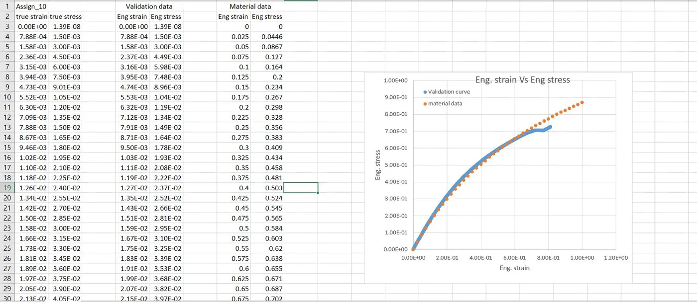
Fig: snapshot of excel sheet showing the calculation of each case where true stress - strain are converted to eng. stress- strain and the data is compared with the provided material data.
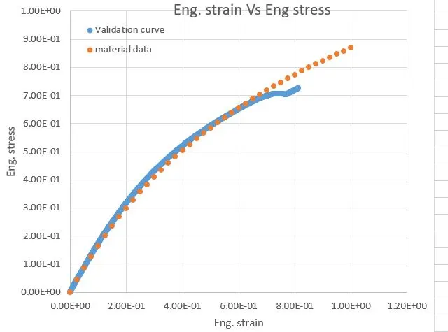
Fig : Comparision of the material data and validation
Conclusion: 1. the Mooney Rivlin and Ogden material constants and compare the both using stress-strain data from a Dogbone specimen tensile test with 100 percent strain.
2. The validation was done to compare with the simulation result and the material data.