Week - 10 Hyperelastic Material Models

AIM:

1. To calculate the Mooney Rivlin and Ogden material constants and compare the both using stress-strain data from aDogbone specimen tensile test with 100 percent strain.
2. The given material data is the engineering stress-strain in MPa/(mm/mm).
3. The comparison should be shown from the d3hsp file and using simulation.

PROCEDURE:

Given Experimental Data:

1. The given data of Engg stress and Engg strain of hyperelastic material is shown in the image given below are plotted in excel.

2. A tensile test model is setup for the given dog-bone model, where the boundary conditions are:
3. a) One end is fixed with all DOFs locked except translation in lateral direction to allow the compression.
4. b) All nodes on the other end are added to a node_set to which a ‘prescribed_boundary_condition’ of displacement is applied in the longitudinal axis.
5. c) The middle node on each of the ends is constrained in all other DOF except translation in the longitudinal axis to avoid contradicting boundary conditions and keep the loading tensile in nature.
6. A linear displacement curve is defined to get cover the experimental test strain which as stated is 100% - the specimen is stretched to twice its original length.
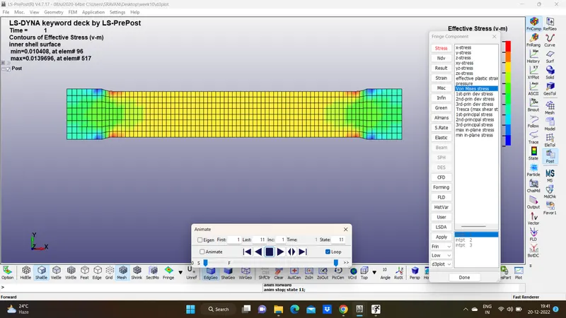
7. The simulation is performed first only to get the hyper-elastic constants for N=1 through N=3. The fitted curve is tested against the input curve as well. Then these constants are used to define the curve emulating the 3 stages and the results arenoted.
8. Finally for the actual simulation for validating the model using the 2 material models mentioned before, the setup is kept the same and the necessary outputs were requested in ‘database’ keyword and the results were compared to the input curves.
9. To understand the process better, implicit analysis is performed.

Analysis Model and setup:

1. Import the dogbone specimen in the working environment.

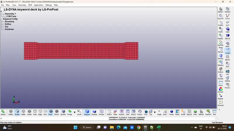
As mentioned, hyper-elastic natural rubber material properties were used for the MAT77 material card. The engineering stress-strain plot was defined using ‘define->curve

1. To verify and validate the given material data with material models of Mooney-Rivlin and Ogden a dogbone specimen is taken for the analysis.

To find the Mooney-Rivlin and Ogden constants the value of N is set to 1-3. The value of density and Poisson’s ratio is taken as the generic value for the rubber material.

The section property of the dogbone specimen is assigned as a shell element with 2 mm thickness and ELFORM=2

1. The Material and Section are assigned to the dogbone specimen part.

Boundary Condition:

1) The nodes at the fixed end are constrained in the X and Z direction only and the Y direction is not constrained because oflateral expansion during the tensile test.

As mentioned above the only boundary conditions defined were the SPCs to make sure the loading is purely tensile, and the prescribed displacement defined with a curve.

1. a) Fixed end with all DOF constrained except lateral translation

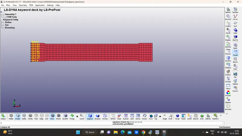
The nodes of the pulling end are assigned with a boundary prescribed motion in X direction using displacement load curve LCID.

Prescribed motion - displacement on the other end for tensile loading:

A linear curve is defined and called upon to impose the boundary condition using a set of nodes the other end from the fixed end.

Control Cards:

1) *CONTROL_IMPLICIT_GENERAL

Activate implicit analysis and define associated control parameters. This keyword is required for all implicit analyses

IMFLAG: Implicit/Explicit analysis type flag: 1- implicit analysis

DT0: Initial time step size for implicit analysis: 0.0100000

IMFORM: Element formulation flag for seamless spring back: 2 retain original element formulation (default)

2) *CONTROL_IMPLICIT_SOLVER

The linear equation solver performs the CPU-intensive stiffness matrix inversion

LSOLVR: Linear equation solver method: 6 (double-precision solver)

3) *CONTROL_IMPLICIT_AUTO card has been defined to adjusts the time step size

IAUTO: set to 1 which automatically adjusts the timestep size.

ITEOPT: optimizes the operation count step:11

ITEWIN: is the iteration window: 5

4) *CONTROL_TERMINATION:

This card is used to mention the termination time of the simulation.

ENDTIM: 1 (Termination time)

5. Analysis setup for Material model validation:

1) The d3hsp file for each material model is opened in notepad++ and the material constants of Mooney-Rivlin and Ogden as well as final fit data of stretch and Engg. stress is obtained for each case.

AFTER TERMINATION CHECK D3HSP FILE

Mooney constant c1 = 0.2224E+00
Mooney constant c2 = 0.8550E-01

For material model validation, the value of N is changed to 3 in the material card. These values are inputted to the material card MAT_77_H. The data obtained from the d3hsp file is an extension (stretch) and True stress which is converted to Engg.strain and Engg, stress to verify with experimental data.

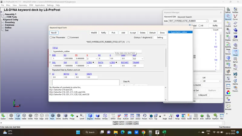
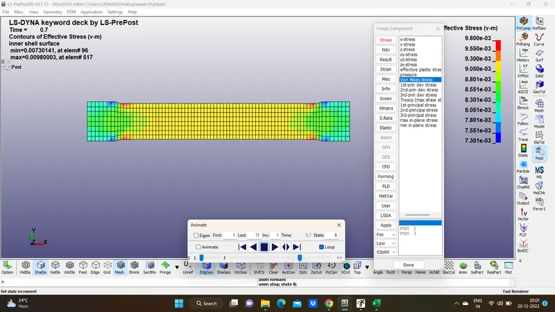
Hyperelastic Constant C10= 0.1660E+00
Hyperelastic Constant C01= 0.1426E+00
Hyperelastic Constant C11= 0.2500E+00
Hyperelastic Constant C20= -0.1130E+00
Hyperelastic Constant C02= 0.6250E-01
Hyperelastic Constant C30= 0.1953E-02

CONCLUSION:

1. The Mooney-Rivlin and Ogden material constants are obtained from d3hsp file by inputting the value of polynomial N=1in the material card MAT_77_H and MAT_77_O
2. The stretch stress curve data obtained from d3hsp for both hyperelastic constitutive models were verified with experimental material data and found to be a close fit.
3. The simulation results of tensile test for both material models with experimental data showed a slight deviation due to high non-linear behaviour of the given hyperelastic material and the generic values of density and Poisson’s ratio.
4. From the simulation results, both hyperelastic constitutive material models were found to be valid to describe the behaviour of the given material data.
5. The Ogden material model has more polynomials ranging from 1 to 8 and is easy to use and gives better adjustment to experimental data at the cost of computional time.
6. Learned to verify and validate hyperelastic material model for the given material data.