Week 1- Mixing Tee

Simulation of T-Joint using RANS based Turbulence Model

INTRODUCTION

The T-Joint is one of the commonly used joints in an Industrial application. Mixing of two fluid at different temperature are of vital importance in the field of nuclear, cryogenic and industrial use where a certain temperature is required as an output, for example mixing of hot and cold fluid to get the desired temperature at the outlet. Mixing of fluid may cause thermals stresses, thermal fatigue in the joint. Moreover how effective is the mixing of two fluids is vitally important for its application.

AIM

The aim of this project is to set up steady-state simulations to compare the mixing effectiveness when the hot inlet temperature is 36⁰C & the Cold inlet temperature is at 19⁰C for short and long T-Joint.

OBJECTIVE

The first objective is to perform the steady-state simulation using k epsilon Realizable and k omega SST based RANS Model. Based on the result of the simulations, one of the models will be selected to compare the mixing effectiveness of T-Joint for different cases.

The different cases of T-Joint are

Case 1

• Short mixing tee with a hot inlet velocity of 3m/s.
• Momentum ratio of 2, 4.

Case 2

• Long mixing tee with a hot inlet velocity of 3m/s.
• Momentum ratio of 2, 4.

where,

Momentum ratio = velocity at cold inlet / velocity at hot inlet

The second objective is to simulate the different cases of T-Joint as mentioned above and draw necessary conclusions.

OUTCOME

1. Compare the following values from the 2 cases:
   • Cell Count
   • Average outlet temperature
   • Number of iterations for convergence
2. Velocity and temperature contour plots on the cut planes along and across the pipe.
3. Velocity and temperature line plots along and across the length of the pipe.
4. Perform Mesh independent study for any one case.
5. Discuss the effect of length and momentum ratio on results.

Geometry Preparation

The steps followed to create geometry in SpaceClaim are as follow

• Import the step file and align the y-axis with the cold fluid inlet pipe.

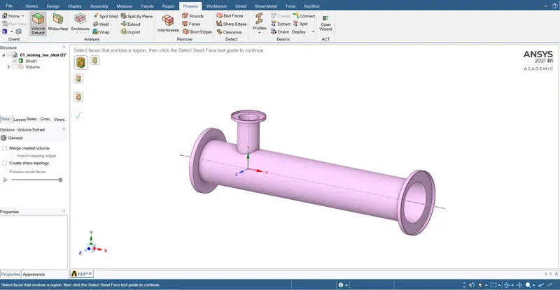
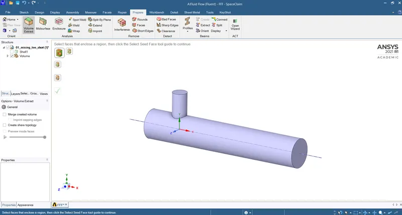
• Use volume extract to create fluid volume as we are interested in fluid mixing. As there is no need to have solid or shell surfaces, so suppress it.

Pre-Processing and Solver Setup

Named Selection, Mesh Preparation, and Mesh Quality Check

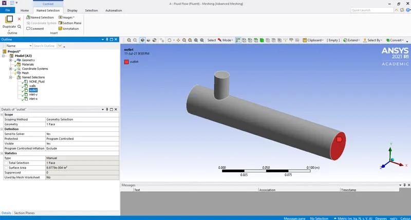
Named Selection is done in the Meshing solver for applying Boundary conditions later in the solver. One of the named selections of outlet is shown in the figure below. Other named selections are shown in the Model tree.

Meshing is done using an element size of 1.25e-3 m and 1.3e-3 m for performing grid dependency test. The figure which shows element size, element quality and element statistics for both the mesh sizes are shown below. While meshing, Automatic Method and Inflation layer are added. Inflation layers with 5 maximum layers with the first layer thickness inflation option are added to capture wall results effectively.

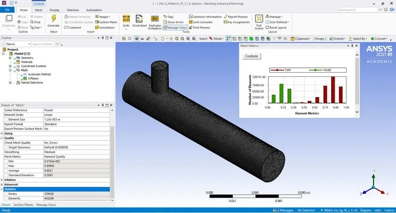
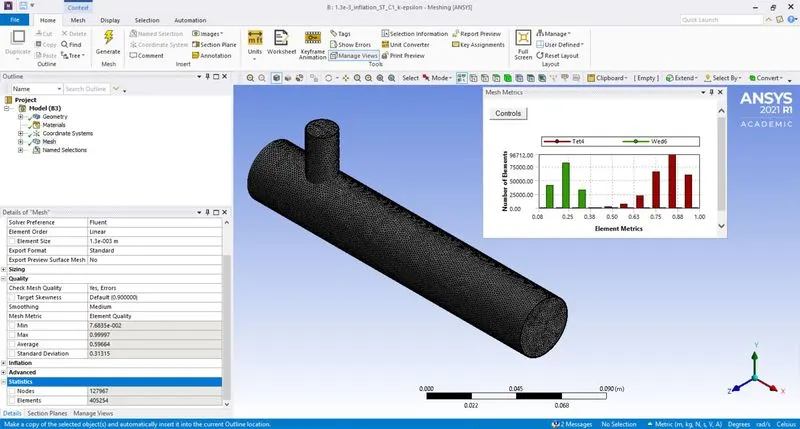
Element Quality Check and Element Statistics

The element quality is sufficient for moving forward with the simulation setup as the minimum element quality in Mesh Metric is greater than 0.05 (minimum element quality permissible) for both the mesh element.

The important details of the Mesh Preparation are shown below in the table

Table-1: Mesh Matrix Table

	Mesh 1	Mesh 2
Element size	1.25e-3 m	1.3e-3 m
Element type	Tet4 and Wed6	Tet4 and Wed6
Element quality (min)	~0.06	~0.08
Nodes	139426	127967
Elements	443299	405254

Solver Setup

Solver setup preparation for one of the subcases of Short T-Joint

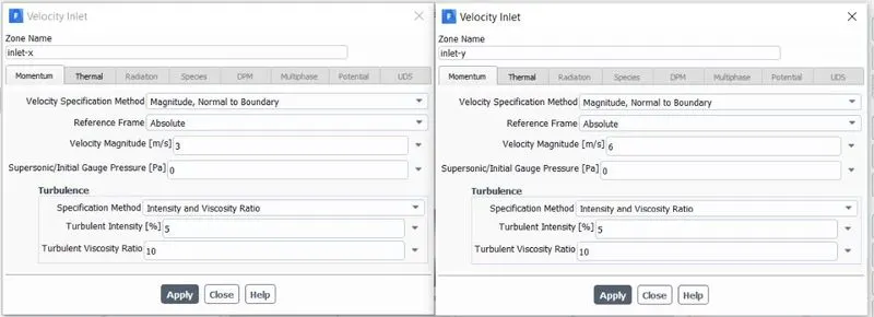
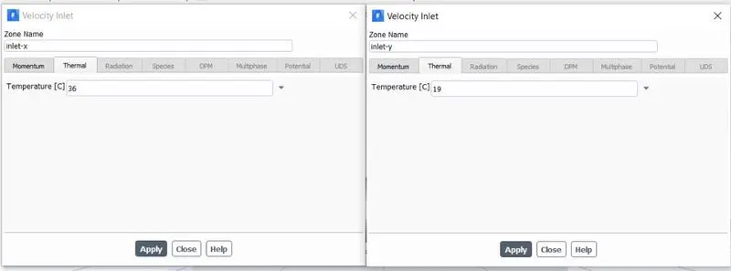
Hot inlet fluid velocity is 3 m/s and temperature is `36^o`C.

Cold inlet fluid velocity is 6 m/s and temperature is `19^o` C.

Other setup details are shown in the table below:

Table-2: Solver setup and boundary conditions details

Setup	Short T-Junction
Solver	Steady-state, Pressure-based, Absolute Velocity Formulation
Fluid Material	Air
Outlet BC	Absolute Pressure
Wall BC	no slip, insulated wall i.e. 0 heat flux

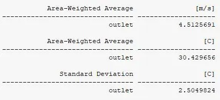
The results of the above case are compared based on the selection of 2 different models i.e. k-epsilon realizable and k-omega SST.

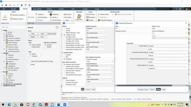
Snippets of the setup preparations for the k-epsilon realizable model are shown below

• Material and Viscous Model selection

• Inlet Boundary conditions for Hot and Cold fluid

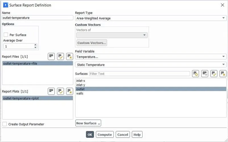
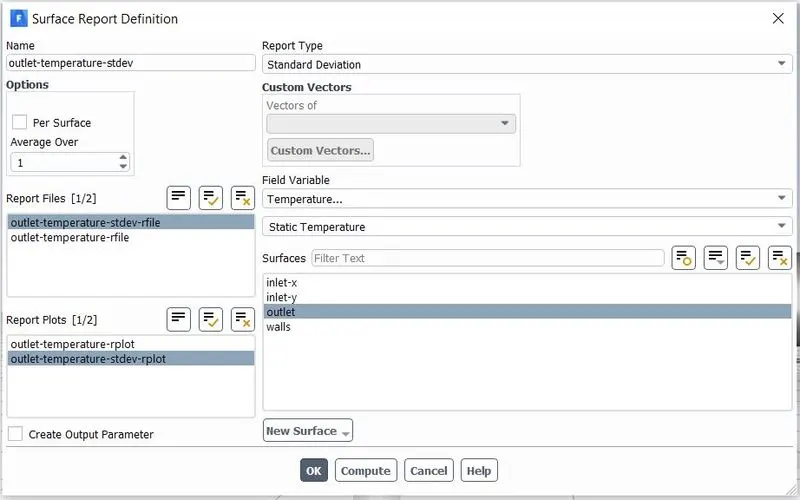
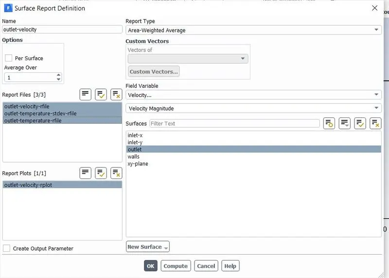
• Snippets of the setup of Area-Weighted average and Standard Deviation of Temperature at the outlet

Results

Grid Dependency Test

Table-3: Grid dependency comparison

	Mesh 1 (1.25e-3 m element size)	Mesh 2 (1.3e-3 m element size)	% change wrt Mesh 2 (absolute)
Converged iteration number	117	116	-
Outlet Velocity	4.509	4.509	0
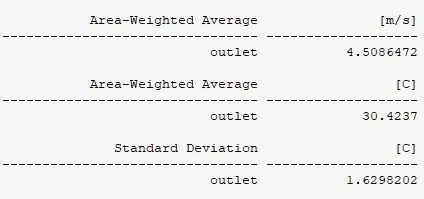
Outlet Temperature	30.425	30.424	0.01
Outlet Temperature standard deviation	1.624	1.630	0.3

Based on the results as shown above, in the table, we can conclude that our results are mesh independent as there are very minute deviations less than 0.05% in the results of outlet velocity, outlet temperature, and the standard deviation of outlet temperature.

For further analysis, 1.3e-3 m element size is considered

• As it is showing less number of iteration took for converging the simulation.
• Outlet temperature standard deviation is also comparable.

Results comparison of k epsilon Realizable and k omega SST model

The comparison is shown for

Case 1: Short Mixing T

Hot inlet velocity 3 m/s, and Cold inlet velocity 6m/s. Other details of the setup are shown in Table-2.

The results of k epsilon and k omega are compared below:

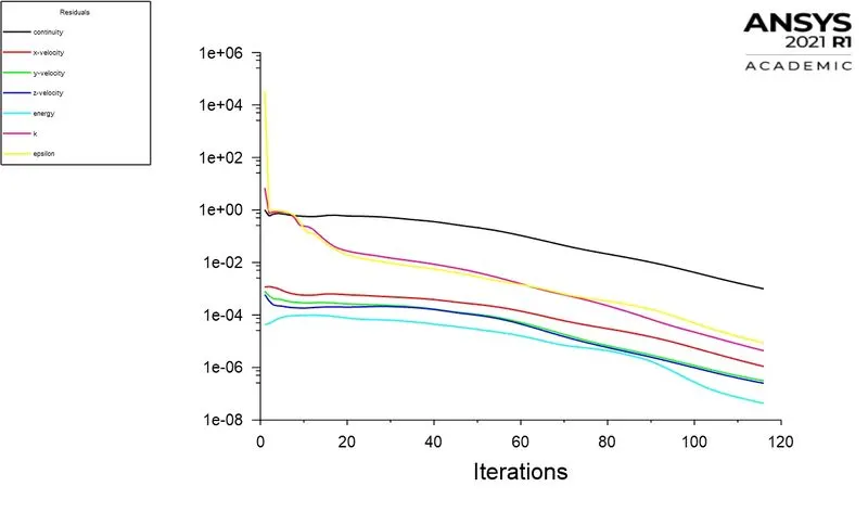
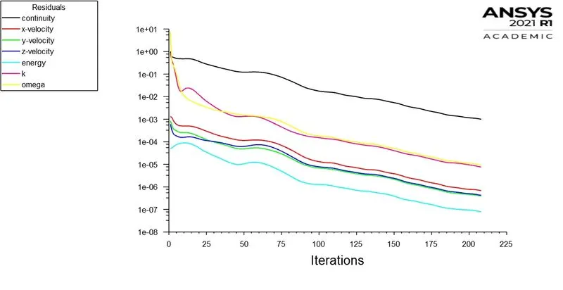
Residuals of the result of k epsilon model simulation.

Residuals of k omega model simulation.

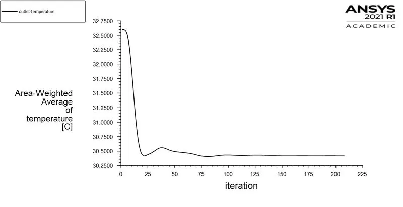
Outlet temperature result of k epsilon model simulation.

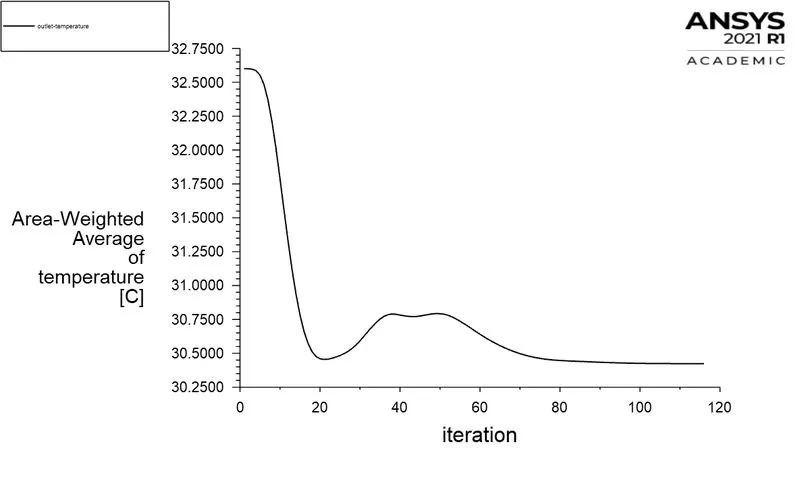
Outlet temperature result of k omega model simulation.

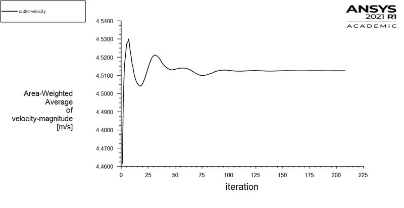
Outlet velocity result of k epsilon model simulation.

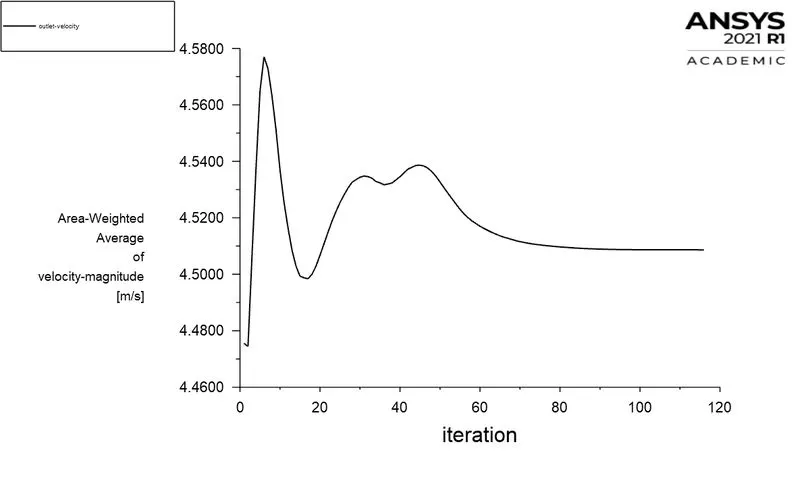
Outlet velocity result of k omega model simulation.

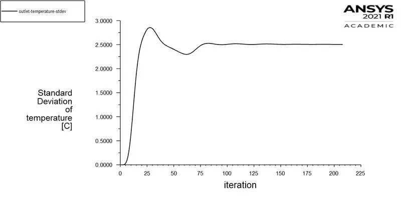
Outlet temperature standard deviation result of k epsilon model simulation.

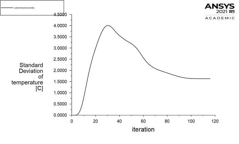
Outlet temperature standard deviation result of k omega model simulation.

Iterations took to converge for k epsilon model simulation.

Iterations took to converge for k epsilon model simulation.

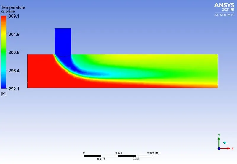
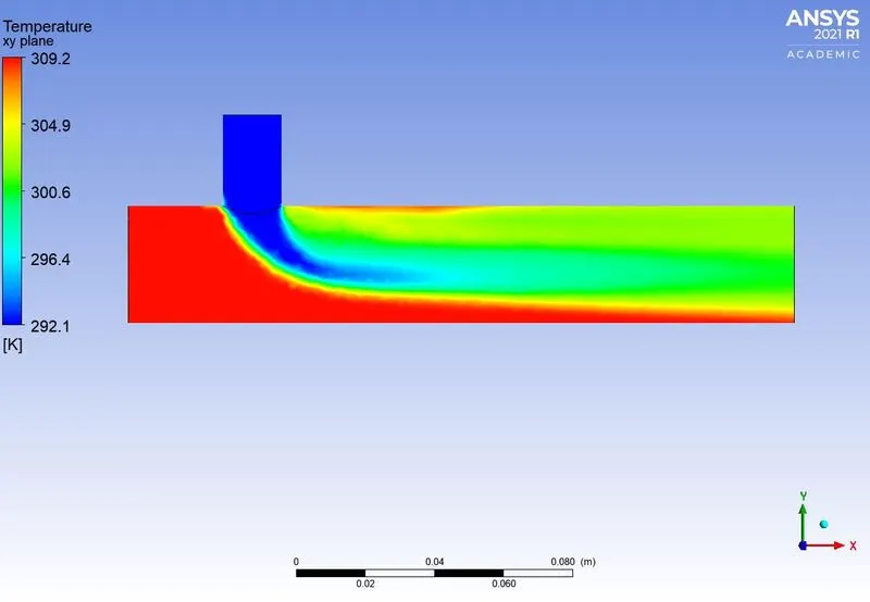
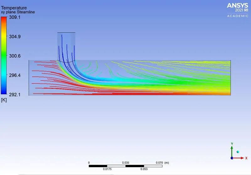
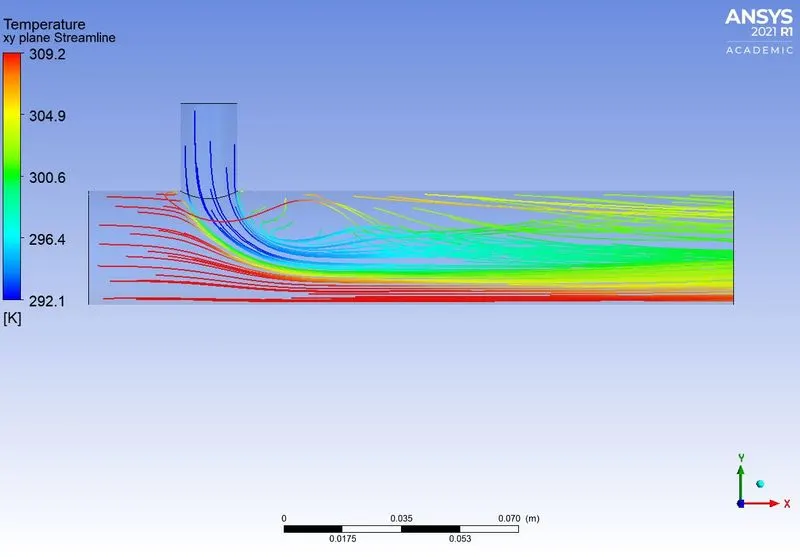
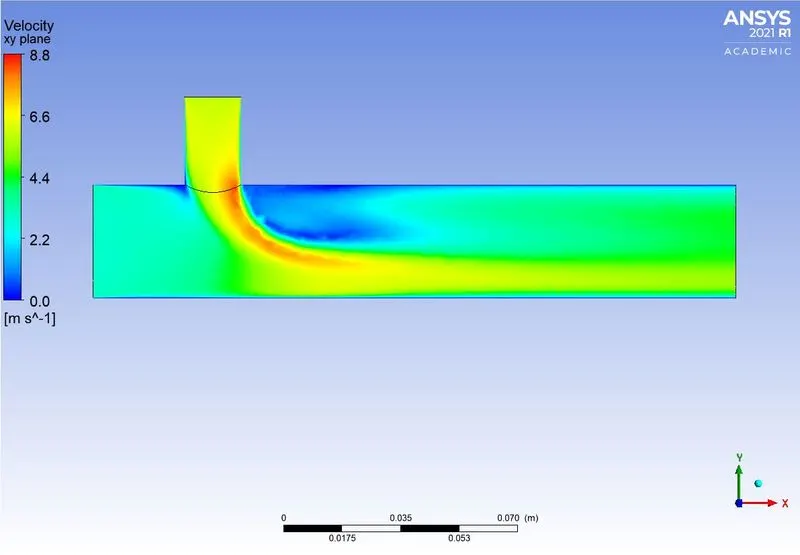
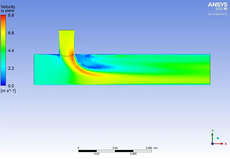
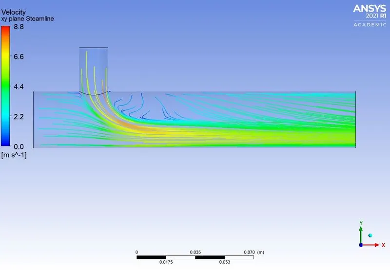
The other results of the k epsilon realizable and k omega SST model are compared side by side below:

Temperature contour and streamline plot result comparison cut along the pipe.

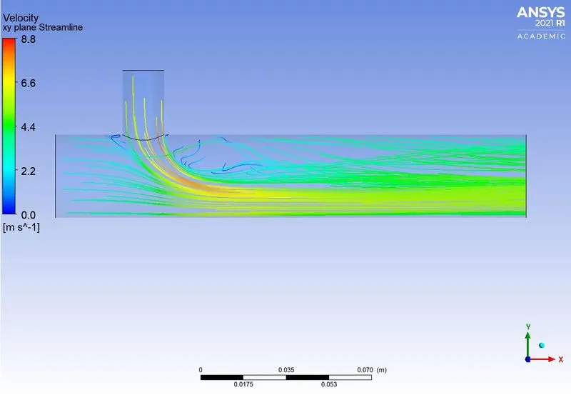
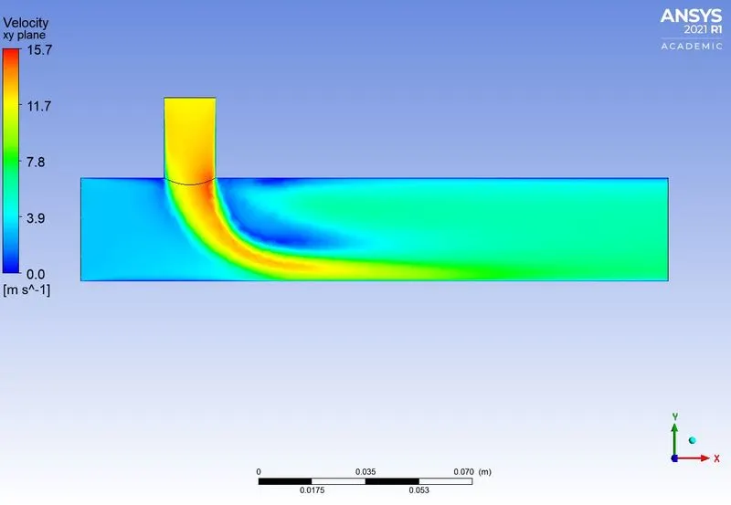
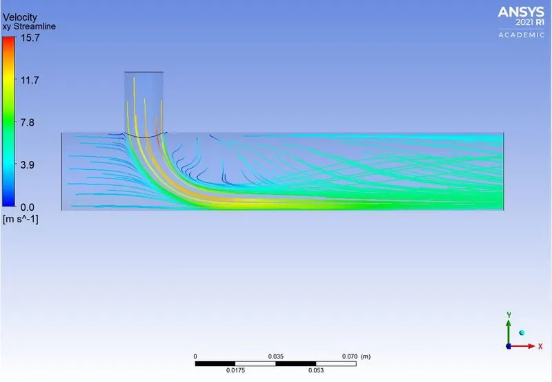
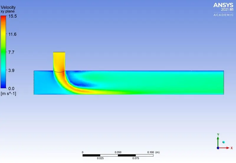
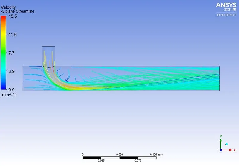
Velocity contour plot and streamline plot result comparison cut along the pipe

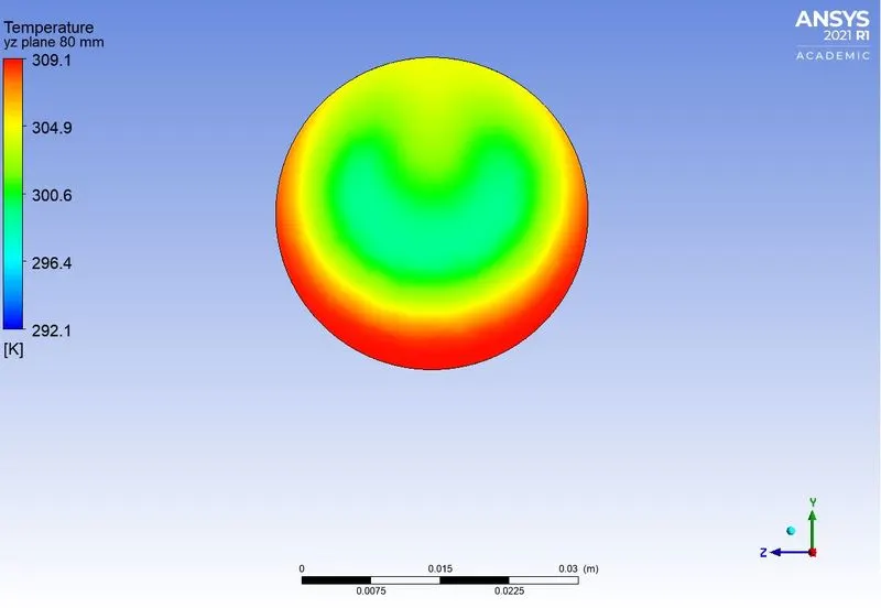
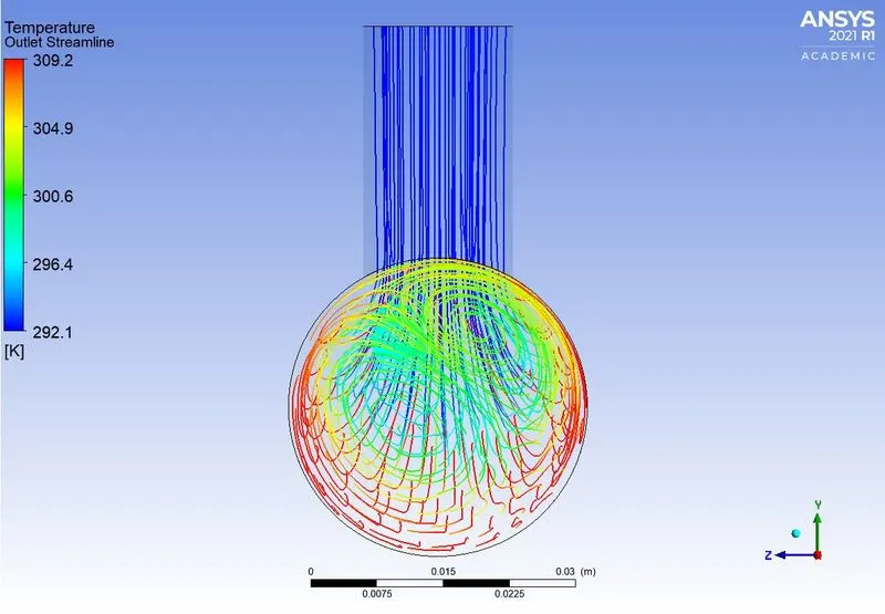
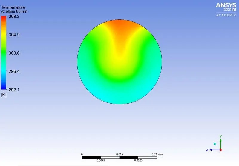
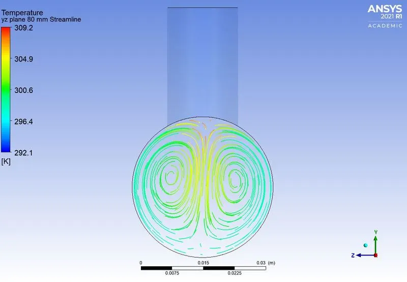
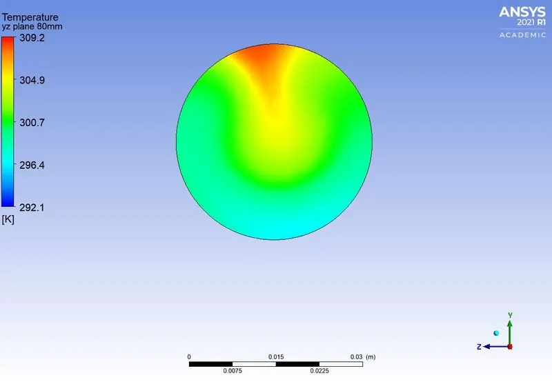
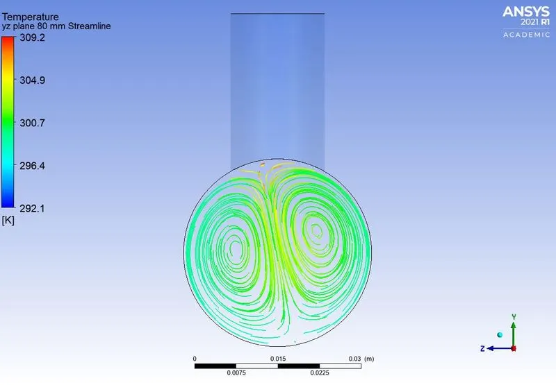
Temperature contour plot and streamline plot result comparison cut across the pipe at 80 mm from cold fluid pipe center axis

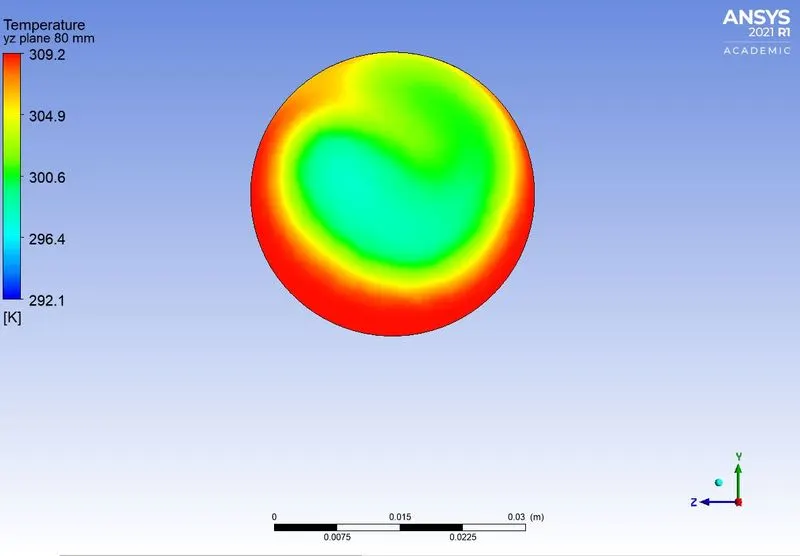
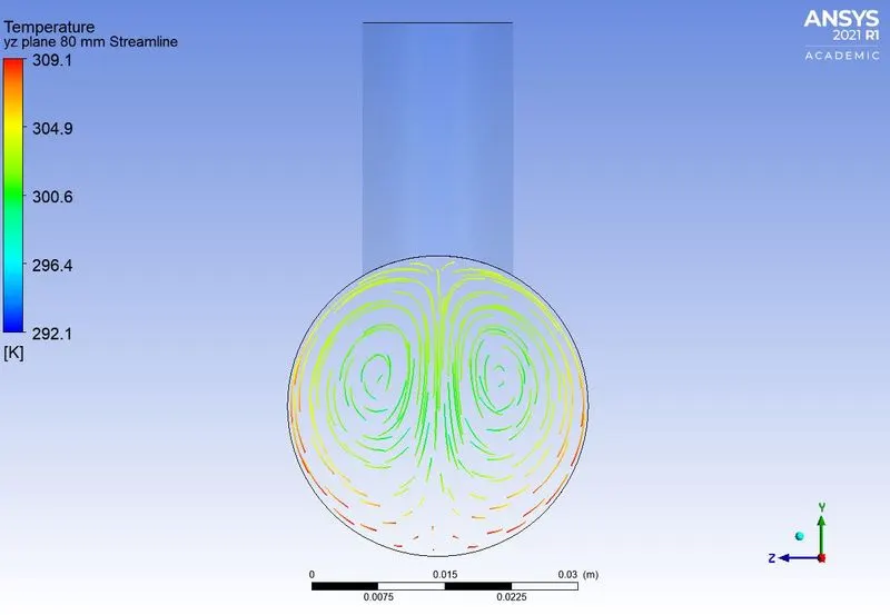
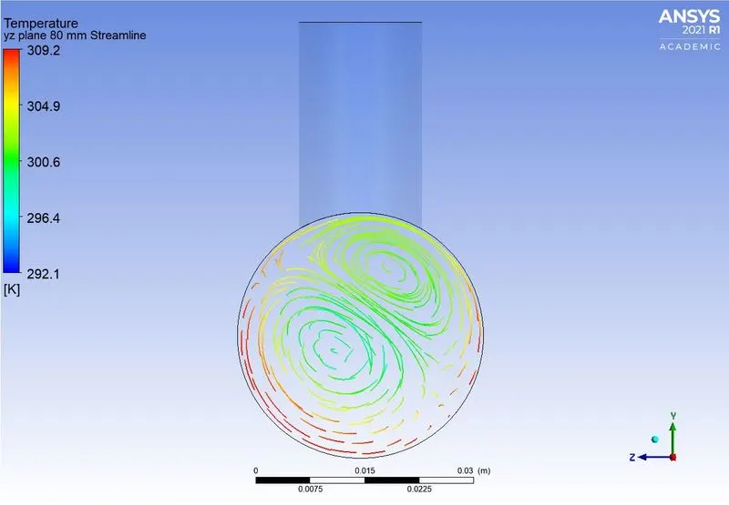
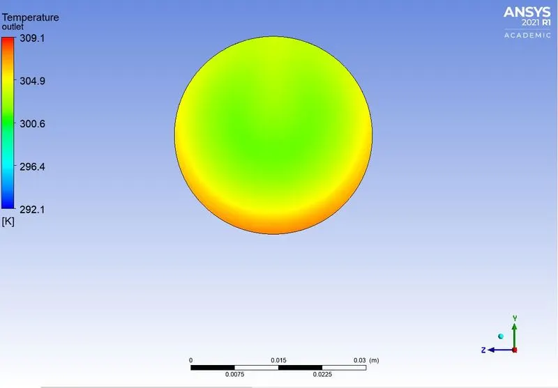
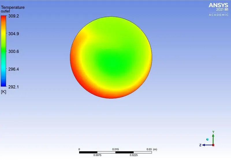
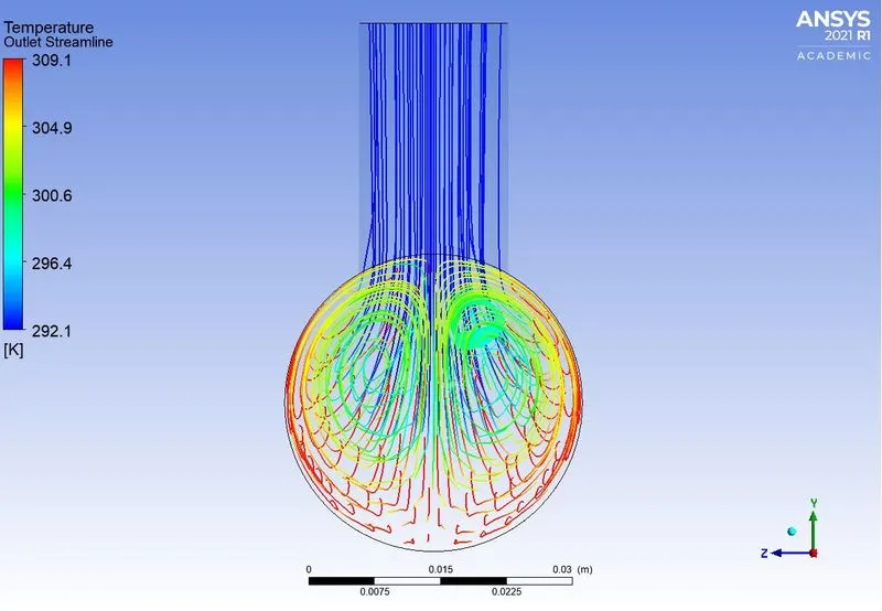
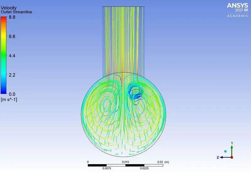
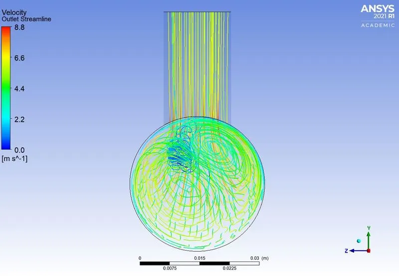
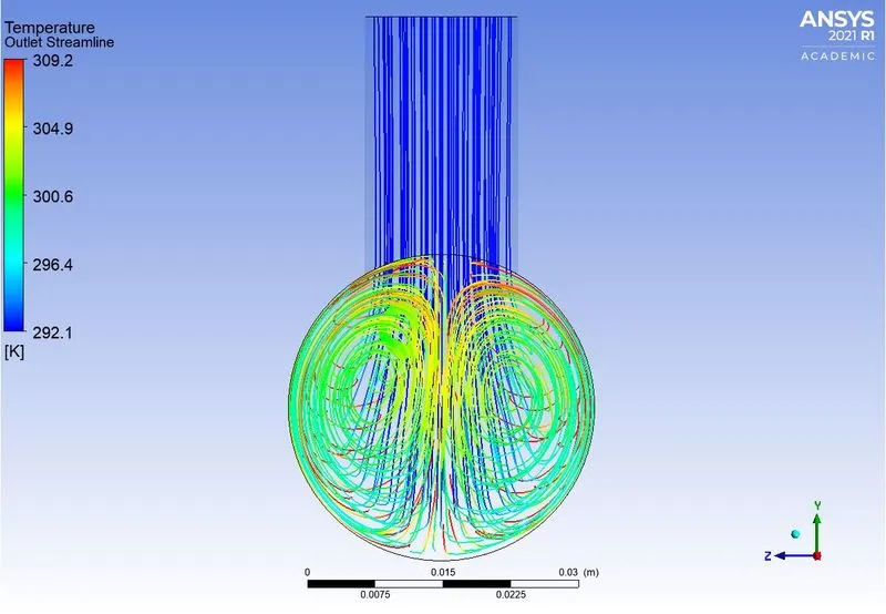
Temperature contour plot and streamline plot result comparison at the outlet cross-section. Here, the streamline direction is taken in backward direction instead of forward in other cases as after outlet there is no streamline plot so we have to plot in the backward direction. for further cases of streamline plot at the outer similar backward direction will be used.

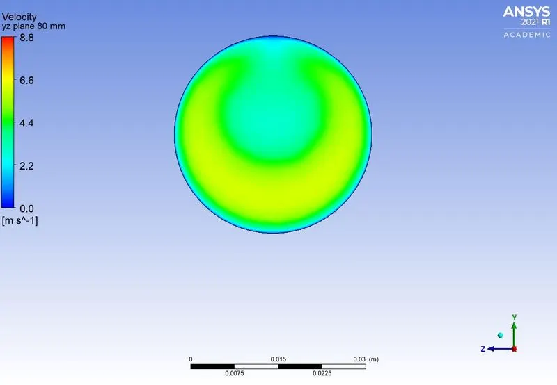
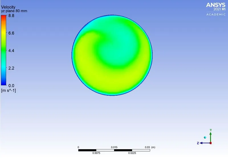
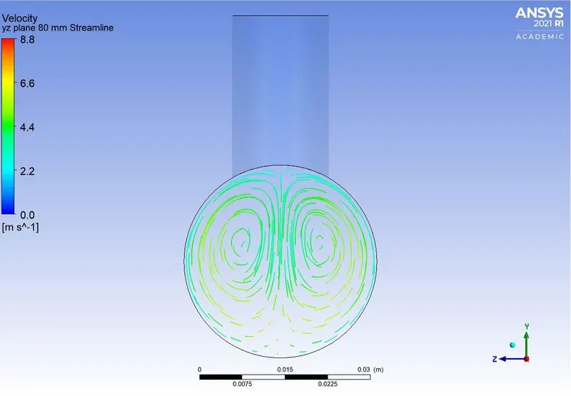
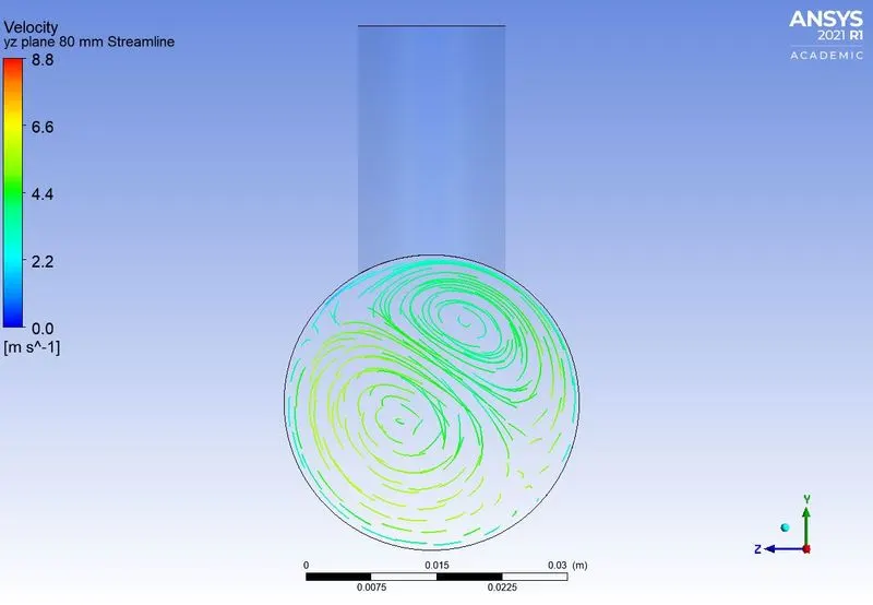
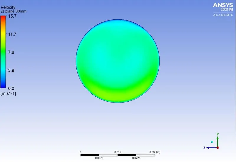
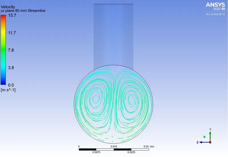
Velocity contour plot and streamline plot result comparison cut across the pipe at 80 mm from cold fluid pipe center axis

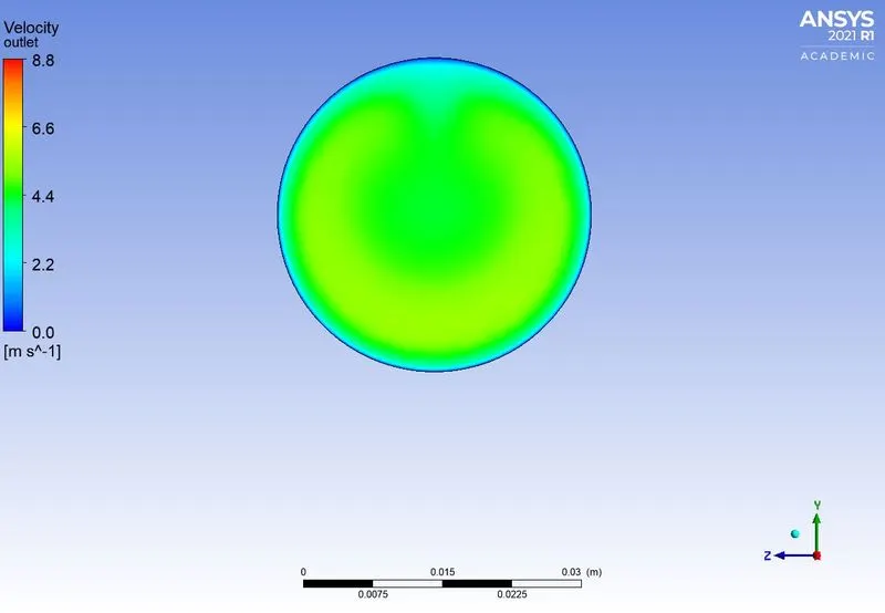
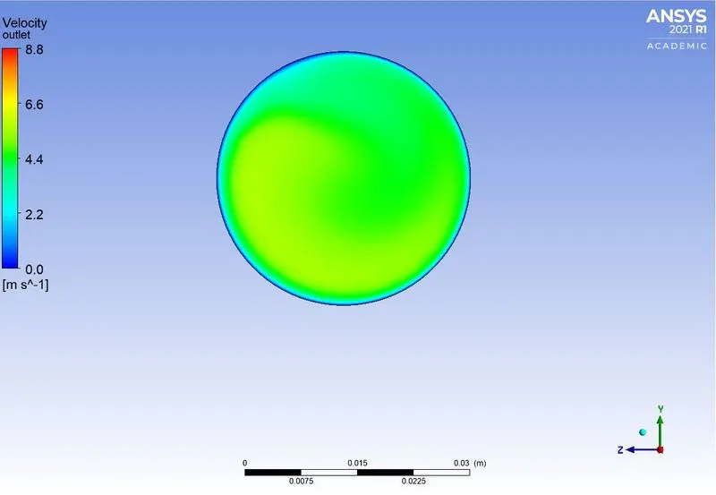
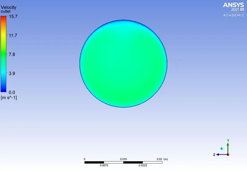
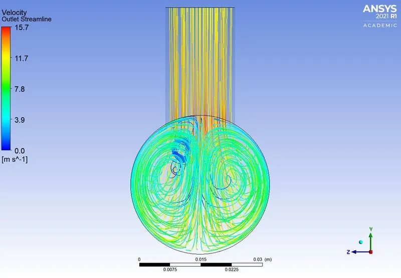
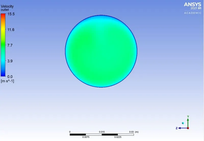
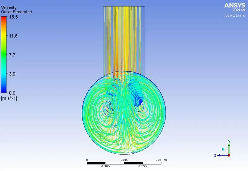
Velocity contour plot and streamline plot result comparison at the outlet cross-section

Conclusions

Based on the simulation performed using k epsilon and k omega following conclusions can be made

• k epsilon model is good for simulating the mixing of two fluids in a T-Joint as it shows better mixing efficiency which is measured by calculating the standard deviation of area-weighted temperature at the outlet.
• The iteration took by the k epsilon model is less than the k omega model. Moreover, the k omega SST model is good for finding out the information near the wall of the pipe and the k epsilon Realizable model is used to find information far away from the pipe walls.
• For further analysis, the k epsilon Realizable model will be used as it shows better mixing efficiency.

Results of other cases with k epsilon Realizable model

Case 2: Short Mixing T

Hot inlet velocity 3 m/s, and Cold inlet velocity 12 m/s. Other details of the model setup are shown in Table 2.

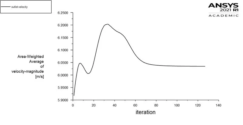
The graphs of residuals and an area-weighted average of temperature, temperature deviation, and velocity at the outlet are shown below:

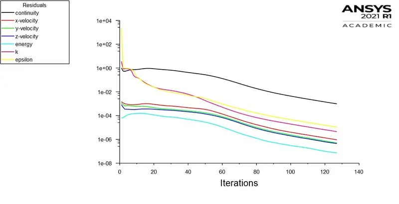
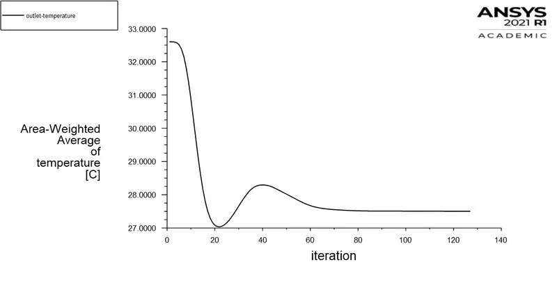
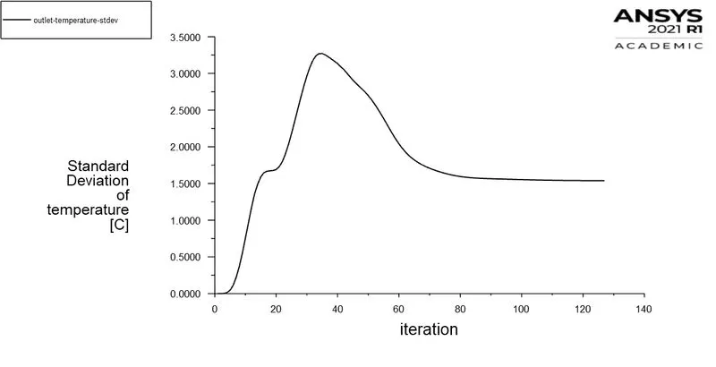
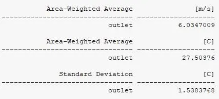
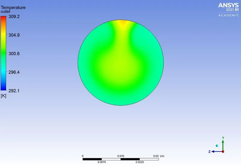
The steady-state results at the outlet of the pipe are shown below.

The number of iteration to converge is shown in the figure below:

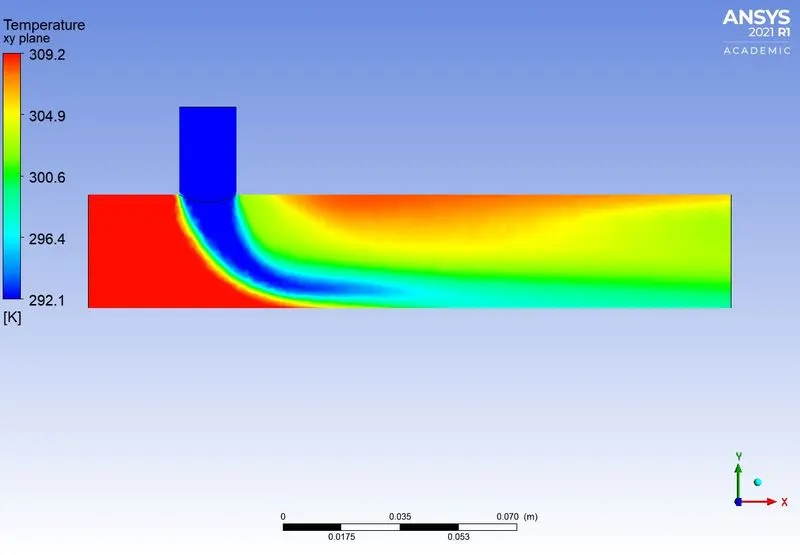
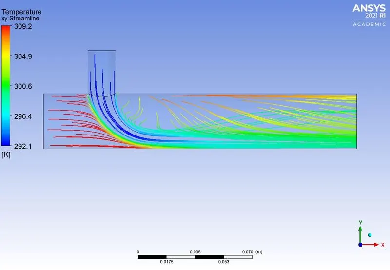
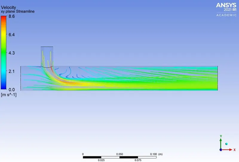
The contour plots and streamline plots of the temperature and velocity along the pipe, across the pipe at 80 mm from the cold fluid center axis and the outlet wall are shown below:

Case 1: Long Mixing T

Mesh Preparation, and Mesh Quality Check

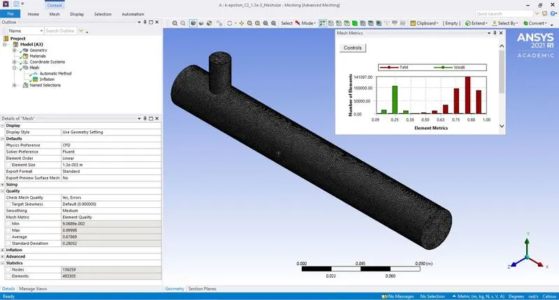
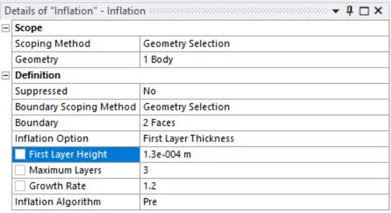
Meshing is done using an element size of 1.3e-3 m. The figure which shows element size, element quality and element statistics for mesh size are shown below. While meshing, Automatic Method and Inflation layer are added. Inflation layers with 3 maximum layers with the first layer thickness inflation option are added to capture wall results effectively. The inflation details are also shown below.

Element Quality Check and Element Statistics

The element quality is sufficient for moving forward with the simulation setup as the minimum element quality in Mesh Metric is greater than 0.05 (minimum element quality permissible).

The important details of the Mesh Preparation are shown below in the table

Table-4: Mesh Matrix Table

	Mesh Details
Element size	1.3e-3 m
Element type	Tet4 and Wed6
Element quality (min)	~0.09
Nodes	136259
Elements	493305

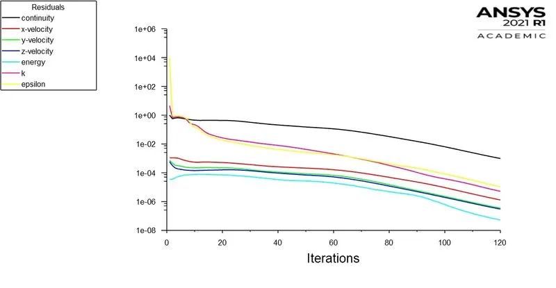
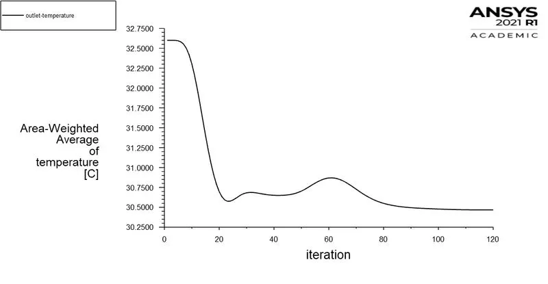
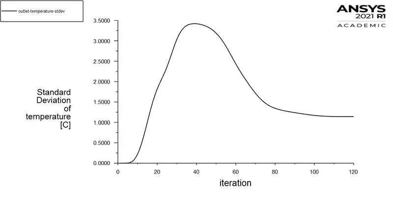
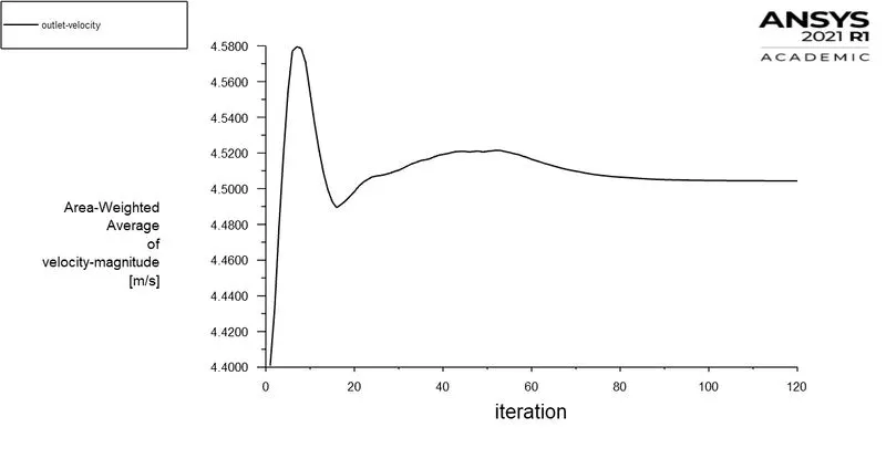
Hot inlet velocity 3 m/s, and Cold inlet velocity 6 m/s. Other details of the model setup are shown in Table 2.

The graphs of residuals and an area-weighted average of temperature, temperature deviation, and velocity at the outlet are shown below:

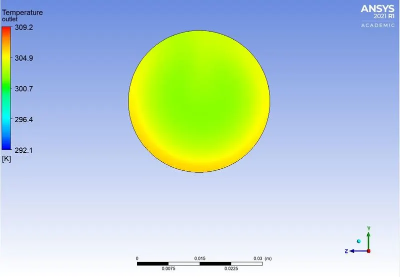
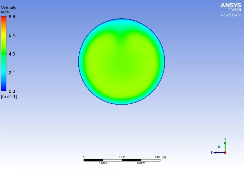
The steady-state results at the outlet of the pipe are shown below.

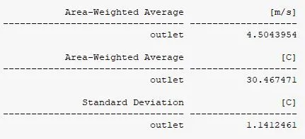
The number of iteration to converge is shown in the figure below:

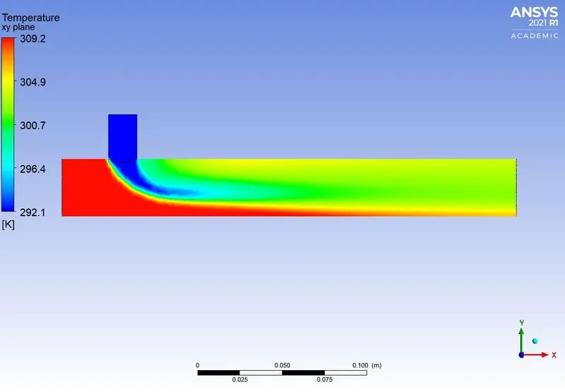
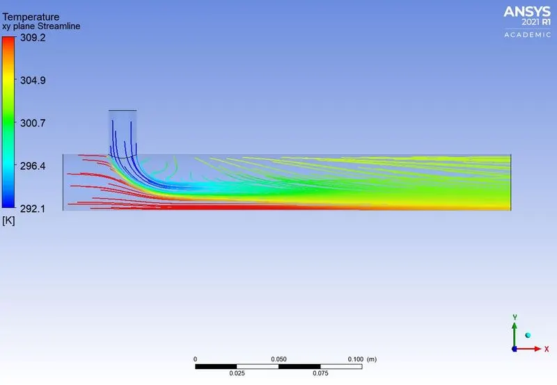
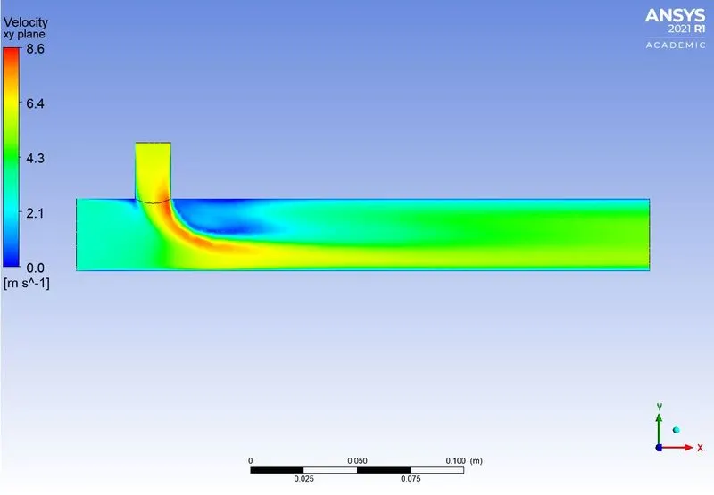
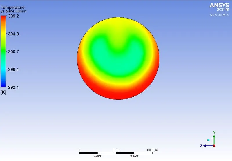
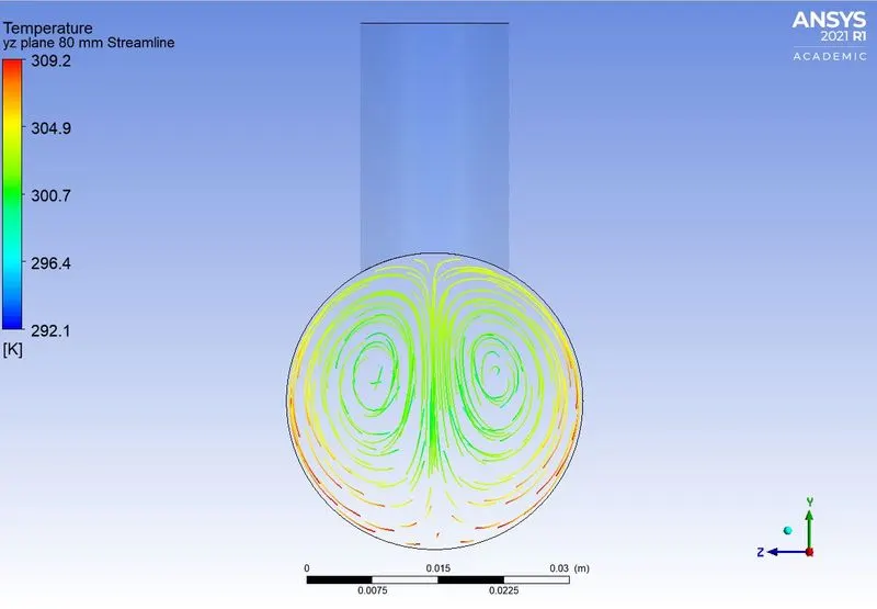
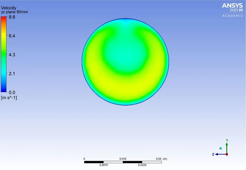
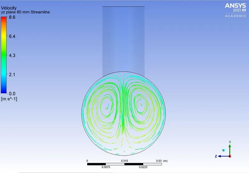
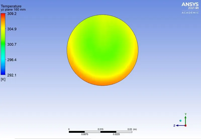
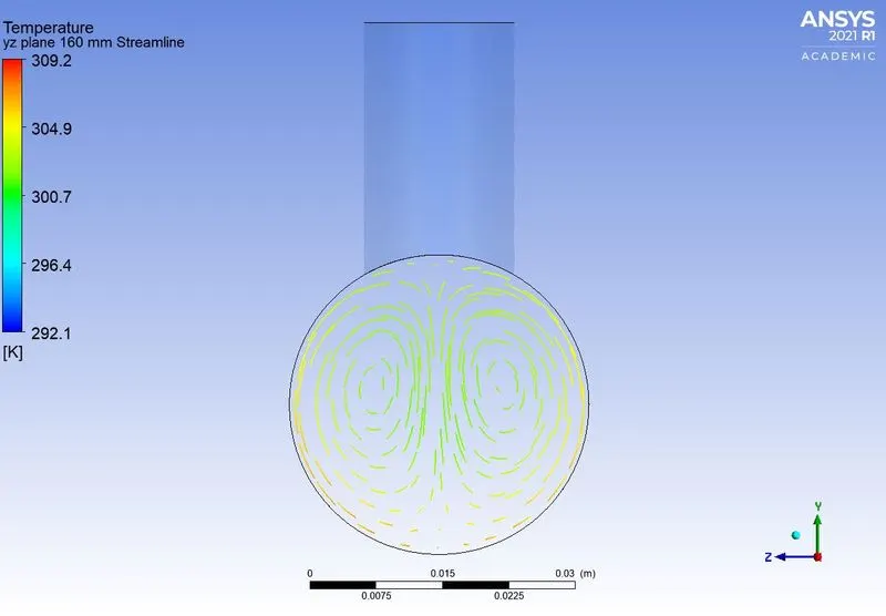
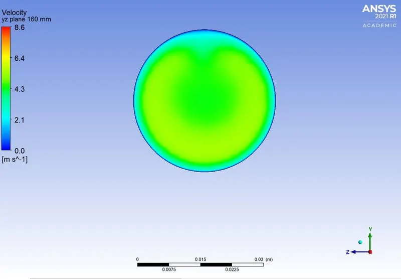
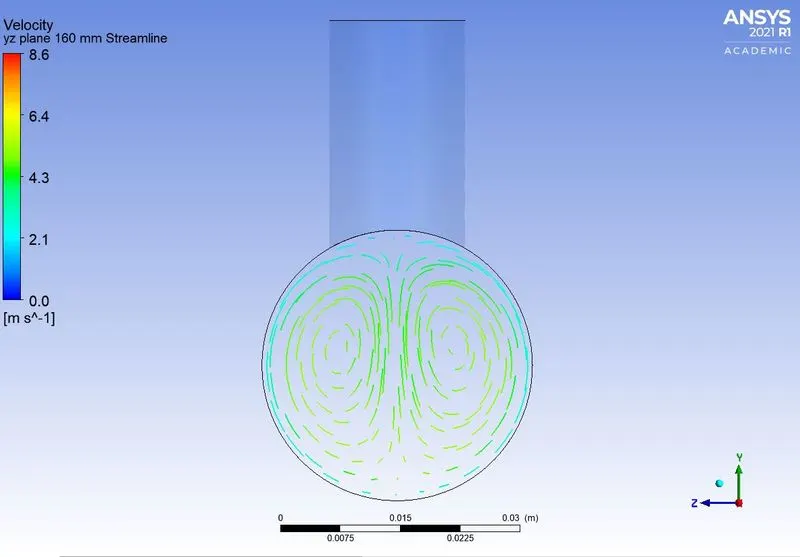
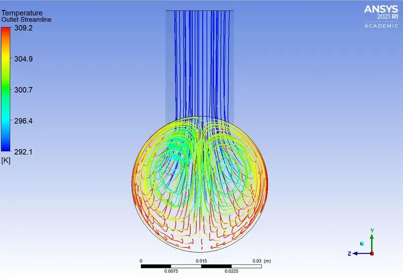
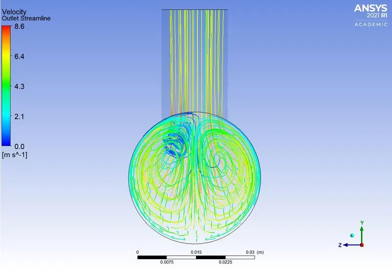
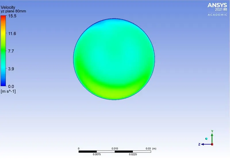
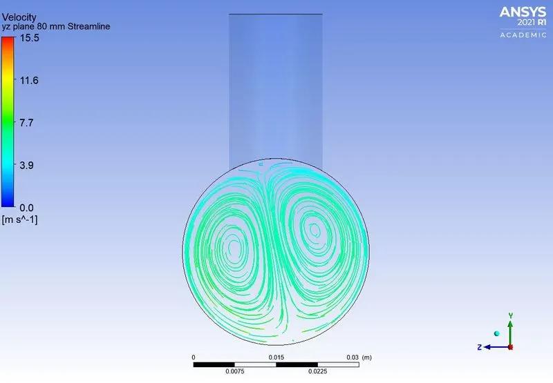
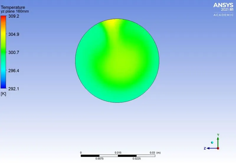
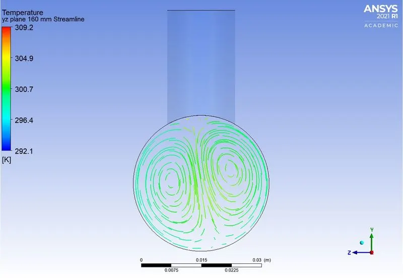
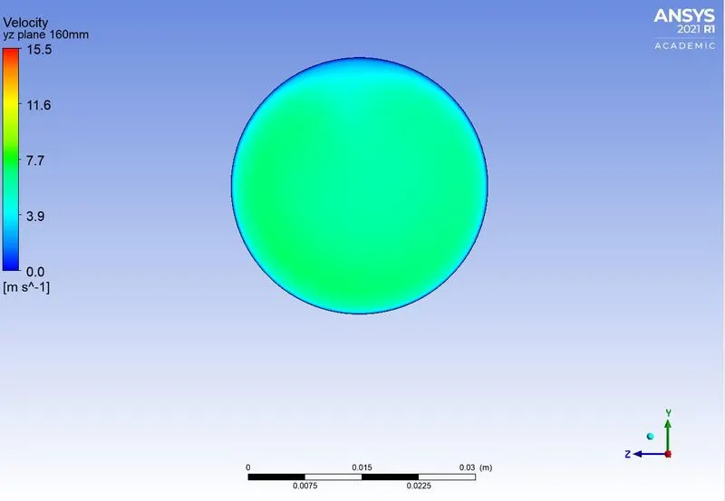
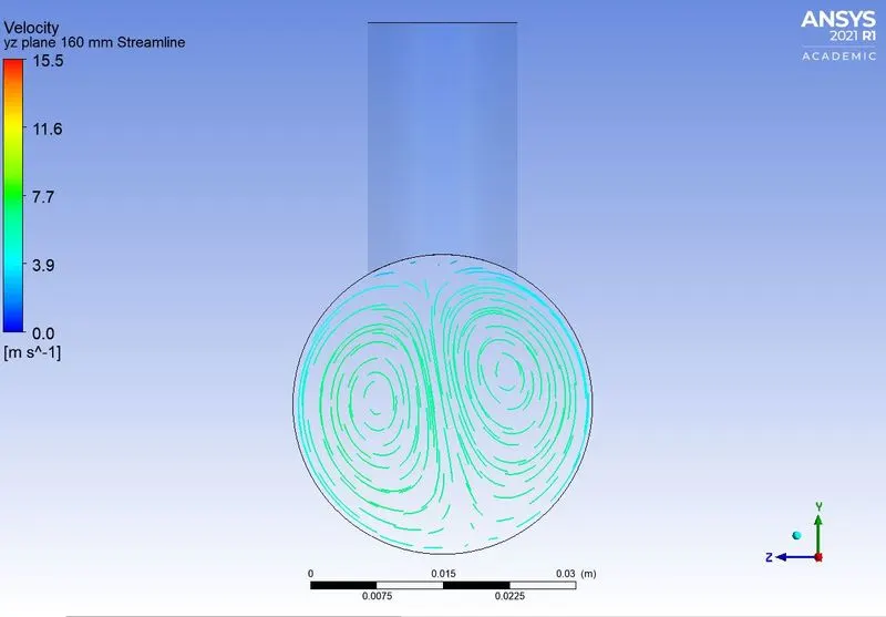
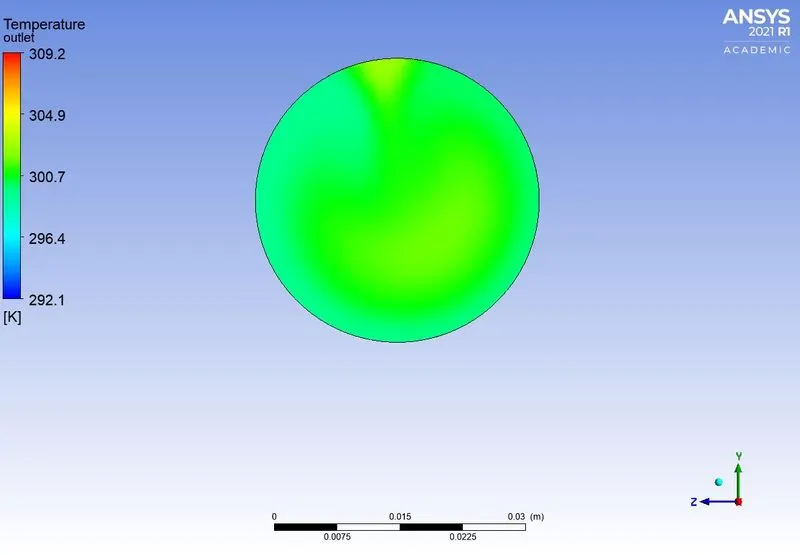
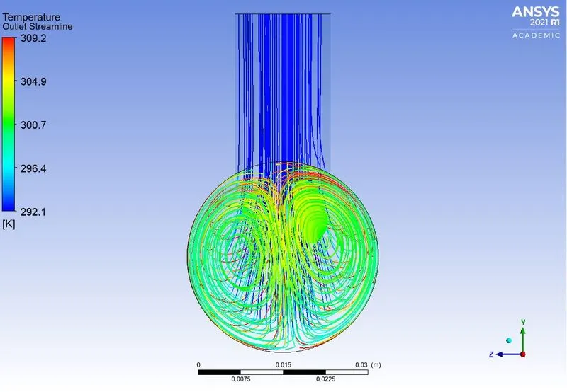
The contour plots and streamline plots of the temperature and velocity along the pipe, across the pipe at 80 mm and 160 mm from the cold fluid center axis and the outlet wall are shown below:

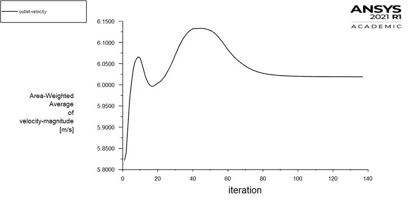
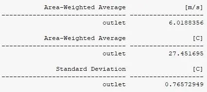
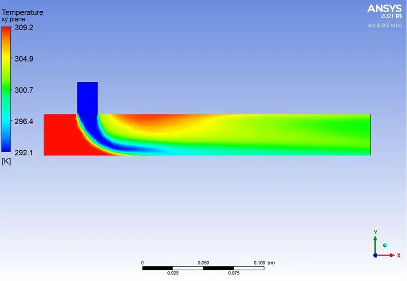
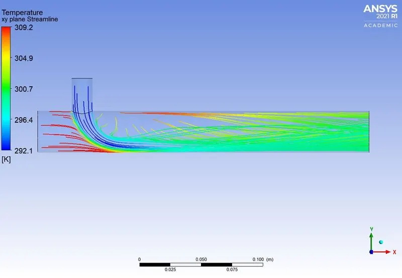
Case 2: Long Mixing T

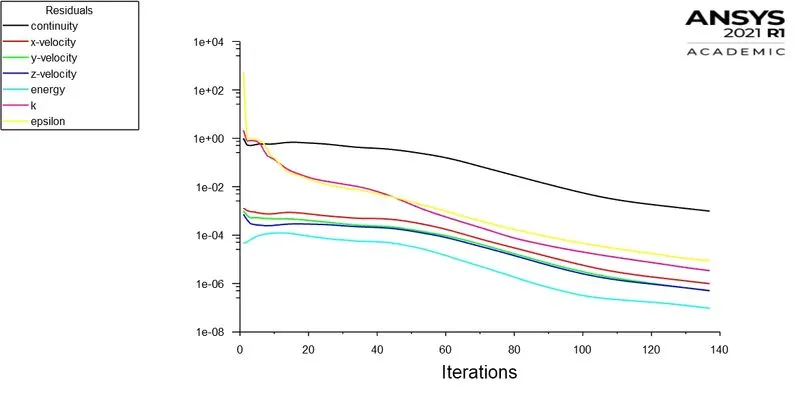
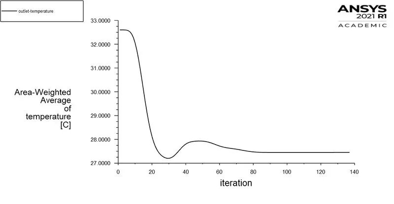
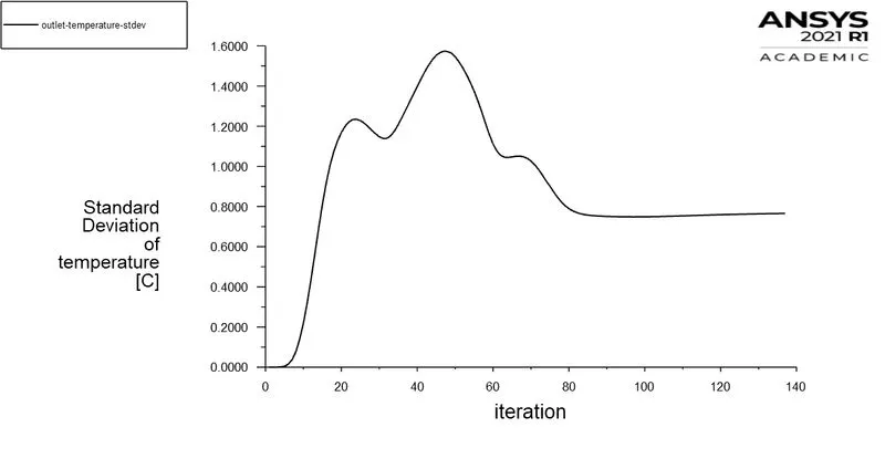
Hot inlet velocity 3 m/s, and Cold inlet velocity 12 m/s. Other details of the model setup are shown in Table 2.

The graphs of residuals and an area-weighted average of temperature, temperature deviation, and velocity at the outlet are shown below:

The steady-state results at the outlet of the pipe are shown below.

The number of iteration to converge is shown in the figure below:

The contour plots and streamline plots of the temperature and velocity along the pipe, across the pipe at 80 mm and 160 mm from the cold fluid center axis and the outlet wall are shown below:

Results Comparison of Short and Long mixing T

Table-5: Results Comparison

	Short Mixing T		Long Mixing T		Short Mixing T	Long Mixing T
	Case 1	Case 2	Case 1	Case 2	Case 1	Case 2
	Simulation	Simulation	Simulation	Simulation	Analytical
Outlet Temperature (C)	30.42	27.50	30.47	27.45	30.32	27.49
Outlet Temperature Standard Deviation (C)	1.63	1.54	1.14	0.77	-	-
Outlet Velocity (m/s)	4.51	6.03	4.50	6.02	-	-
No. of iteration for convergence	116	127	120	137	-	-
Elements	405254		493305		-	-

The analytical formula used to compare the results is `T_(mixture)=(m_(hot)T_(hot)+m_(cold)T_(cold))/(m_(hot)+m_(cold))`

Conclusions

1. The analytical and simulated results of outlet temperature of both the cases of Mixing T Short and Long are quite comparable.
2. On comparing the area-weighted standard deviation of temperature at the outlet, it is observed that Long Mixing T has less standard deviation for both cases simulated for Short and Long Mixing T.
3. The lesser the standard deviation of temperature at the outlet, the better the mixing efficiency of two fluids in the T joint. As the velocity increases of the cold fluid for respective cases, a better mixing efficiency is observed. Thus higher momentum ratio ensures better mixing efficiency.
4. With the increase in the cold fluid velocity increasing the momentum ratio, a drop in the temperature is observed at the outlet.
5. The length of the pipe does not have any impact on the outlet temperature.
6. T joint of longer length ensures better mixing efficiency as it can be seen from the contour plot of temperature and velocity along and across the pipe length. In the case of longer pipes, it is quite evident that better results are observed right from the location across the pipe at 160 mm from the cold fluid center.

The link of video animation of temperature and velocity of all the cases for short and long mixing T using k epsilon realizable model are attached below:

Short Mixing T

Case 1

Temperature video link:

Velocity video link:

Case 2

Temperature video link:

Velocity video link:

Long Mixing T

Case 1

Temperature video link:

Velocity video link:

Case 2

Temperature video link:

Velocity video link: