Week 1- Mixing Tee

AIM

Case study of simulation of internal flow through mixing tee tube using Ansys Fluent.

INTRODUCTION

In this case study we are going to study internal flow of two fluids at different temperature through mixing tee tube and study the temperature and velocity at outpt of mixing tee tube under different conditions like mesh parameter,velocity and momentum ratio.

Theory Of Topics

1.)Mixing Tee Tube

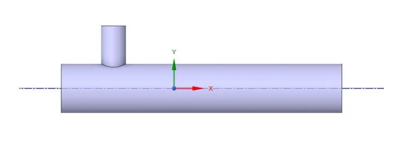
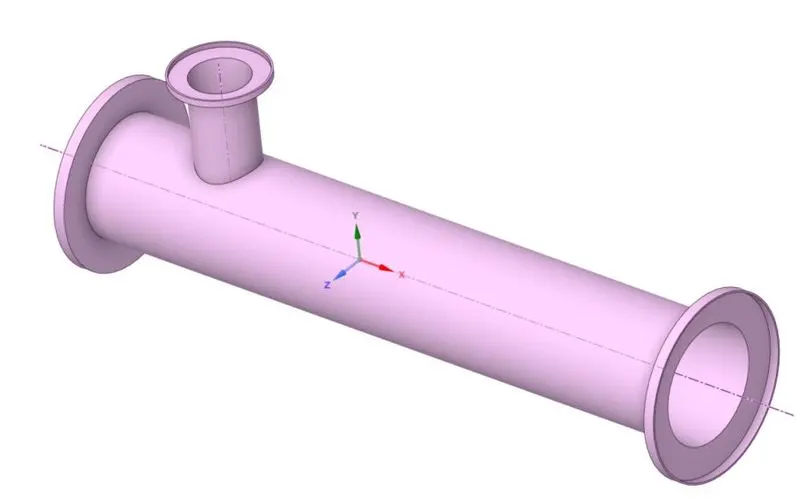
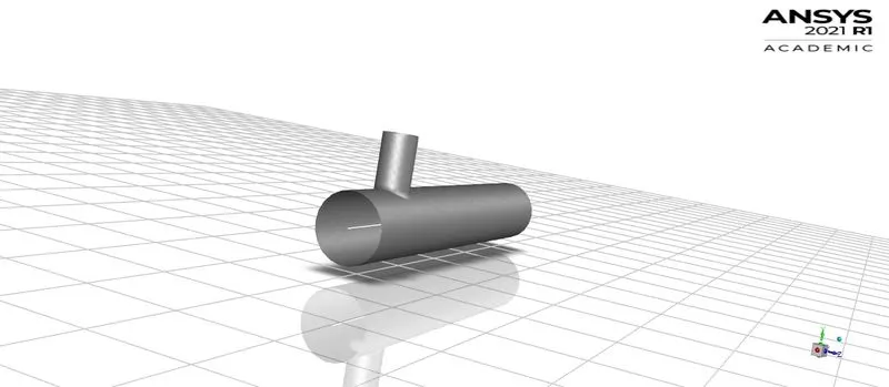
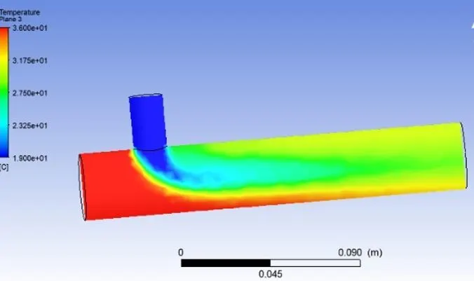
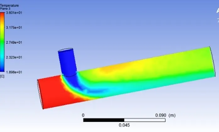
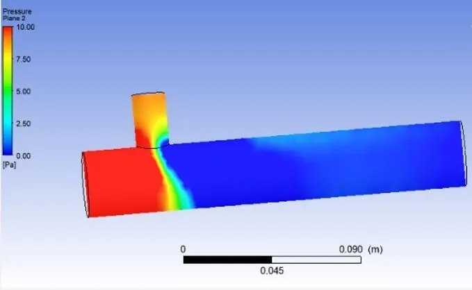
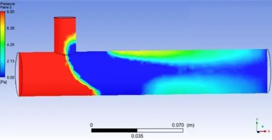
Mixing Tee is the combination of two pipes which is joined at an angle of 90 degree (ie perpendicular) ,one type of fluid is passed through the one side of pipe which is horizontal and another fluid is passed through the pipe which is perpendicular to the straight pipe,output is measuerd at another side of straight pipe (As shown in below picture).

2.)Momentum ratio

Momentum ratio: It is defined as a ratio of velocity at the cold inlet to the velocity at the hot inlet(Dimensionless quantity).

Mr = velocity at cold inlet/velocity at hot inlet

3.)K EPSILON(Source Internet)

The k-epsilon (k−ϵ) model for turbulence is the most common to simulate the mean flow characteristics for turbulent flow conditions. It belongs to the Reynolds-averaged Navier Stokes (RANS) family of turbulence models where all the effects of turbulence are modeled.

It is a two-equation model. That means that in addition to the conservation equations, it solves two transport equations (PDEs), which account for the history effects like convection and diffusion of turbulent energy. The two transported variables are turbulent kinetic energy (k), which determines the energy in turbulence, and turbulent dissipation rate (ϵ), which determines the rate of dissipation of turbulent kinetic energy.

The k−ϵ model is shown to be reliable for free-shear flows, such as the ones with relatively small pressure gradients, but might not be the best model for problems involving adverse pressure gradients, large separations, and complex flows with strong curvatures.

4.) k OMEGA(Source Internet)

The k-omega (k−ω) turbulence model is one of the most commonly used models to capture the effect of turbulent flow conditions. It belongs to the Reynolds-averaged Navier-Stokes (RANS) family of turbulence models where all the effects of turbulence are modeled.

It is a two-equation model. That means in addition to the conservation equations, it solves two transport equations (PDEs), which account for the history effects like convection and diffusion of turbulent energy. The two transported variables are turbulent kinetic energy (k), which determines the energy in turbulence, and specific turbulent dissipation rate (ω), which determines the rate of dissipation per unit turbulent kinetic energy. ω is also referred to as the scale of turbulence.

The standard k−ω model is a low Re model, i.e., it can be used for flows with low Reynolds number where the boundary layer is relatively thick and the viscous sublayer can be resolved.

Thus, the standard k−ω model is best used for near-wall treatment. Other advantages include a superior performance for complex boundary layer flows under adverse pressure gradients and separations (e.g., external aerodynamics and turbomachinery). On the contrary, this model has also shown to predict excessive and early separations.

Difference (Source Internet)

K epsilon	K omega
Turbulent Energy k	Turbulent Energy k
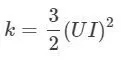
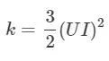
turbulence intensity	turbulence intensity
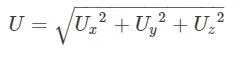
mean velocity U	mean velocity U
turbulent dissipation rate	turbulent dissipation rate
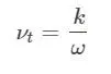
turbulent viscosity νt	turbulent viscosity νt

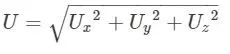
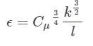
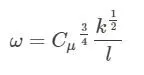
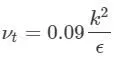
Short Pipe

Case 1:

• Short mixing tee with a hot inlet velocity of 3m/s.
• Momentum ratio of 2, 4.

Momentum ratio = velocity at cold inlet/velocity at hot inlet 1.)Momentum ratio of 2 2= velocity at cold inlet/ velocity at cold inlet=6m/s 2.)Momentum ratio of 4 4= velocity at cold inlet/ velocity at cold inlet=12m/s

Properties		V (inlet x)		V (inlet y)
Turbulence Model		k- ϵ		k- ϵ
Velocity of Hot Inlet		3m/s		3m/s
Hot Inlet Temperature		36 ˚C		36 ˚C
Cold Inlet Temperature		19 ˚C		19 ˚C

Long Tube

Case 2:

• Long mixing tee with a hot inlet velocity of 3m/s.
• Momentum ratio of 2, 4.

Momentum ratio = velocity at cold inlet/velocity at hot inlet 1.)Momentum ratio of 2 2= velocity at cold inlet/ velocity at cold inlet=6m/s 2.)Momentum ratio of 4 4= velocity at cold inlet/ velocity at cold inlet=12m/s

Properties		V (inlet x)		V (inlet y)
Turbulence Model		k- ϵ		k- ϵ
Velocity of Hot Inlet		3m/s		3m/s
Hot Inlet Temperature		36 ˚C		36 ˚C
Cold Inlet Temperature		19 ˚C		19 ˚C

Importance in Practical Application

1.)Petrochemical Industry where two fluid stream with differnt physical and chemical properties is mixed.

2.)HVAC Industry

3.)Chemical Engeneering Industry

4.)Wastewater treatment

5.)Injection of aditives

Solving and Modelling Approach

1.)Upload the model

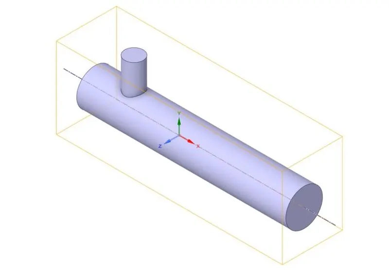
2.)extract the volume as temperature and velocity is measured not on surface

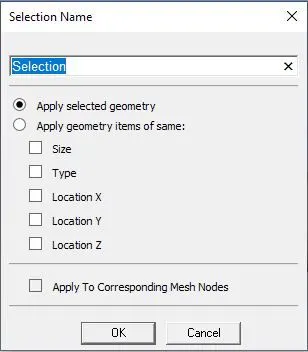
3.)Naming (inlet,outlet and walls)

4.)Meshing(standard or change size as required)

5.)Element quality (grater than than 5%)

6.)Update the model in solver

7.)Run Mesh quality checker

8.)Define domain,physical properties, defination.covergence ,iteration and initialize

9.)calculate

10.)check for graphs and plots

11.)check for simulation result

Pre Process

The pre process for both case is explained with short pipe example

Case 1:

• Short mixing tee with a hot inlet velocity of 3m/s.
• Momentum ratio of 2, 4.

Case 2:

• Long mixing tee with a hot inlet velocity of 3m/s.
• Momentum ratio of 2, 4.

Geometry:

Extracted volume:

Meshed :

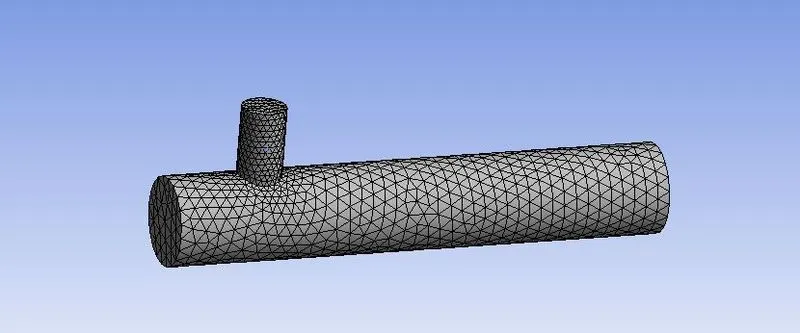
Sectional View of Meshed Pipe:

Pipe opened in Solver

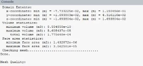
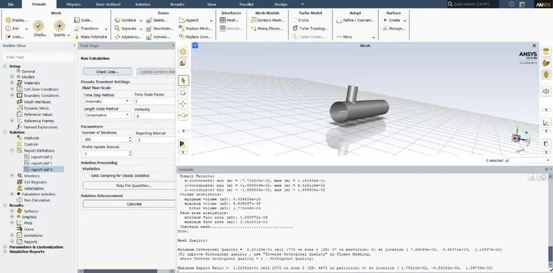
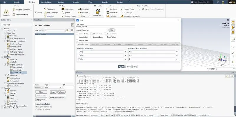
Mesh Quality Checker

Console

Case 3:

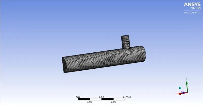
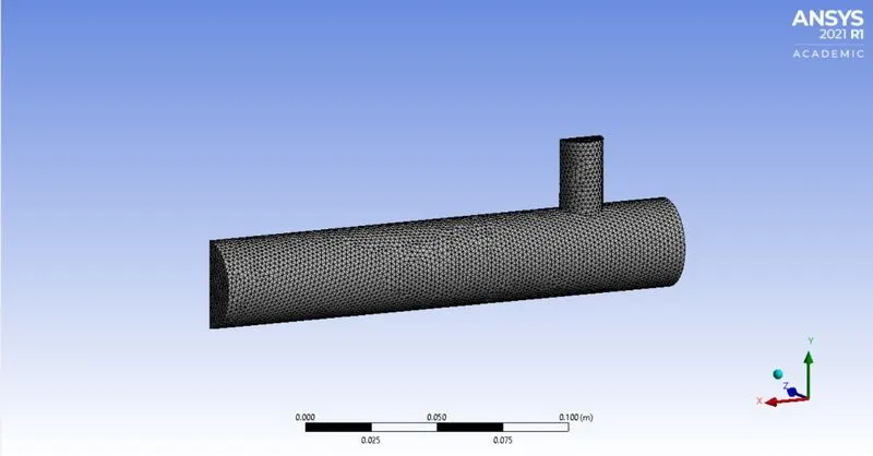
Different Mesh size

Mesh sixe0.003

Mesh sixe0.002

Short tee (ratio 4)	Mesh size	Nodes	Elements
	0.003	8,345	39,808
	0.002	21,344	1,05,860

RESULTS:

Case1:

Short tee momentum ratio 2:

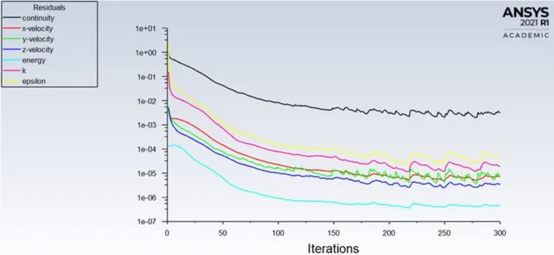
Residuals:

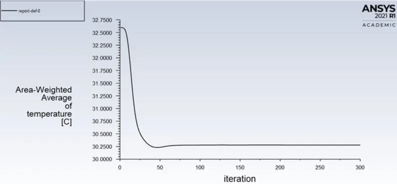
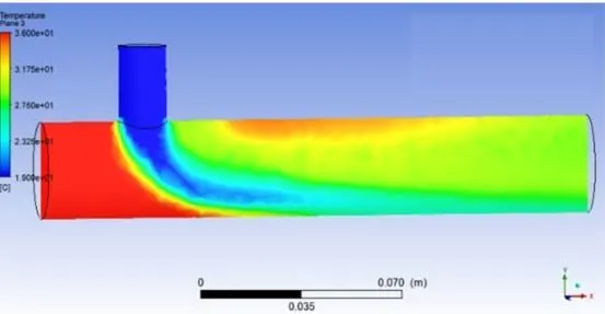
Temperature at outlet:

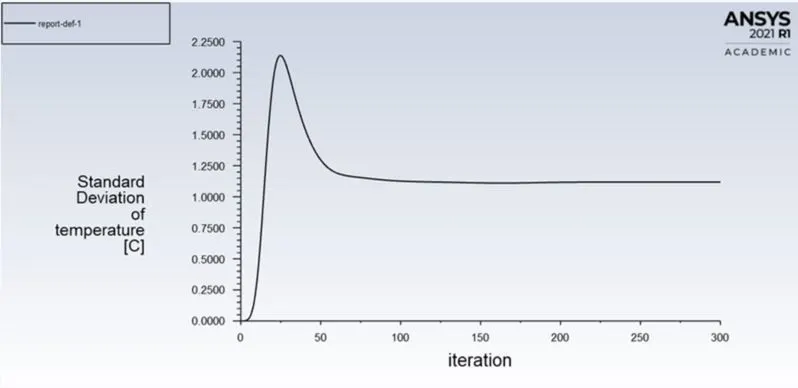
Standard deviation of temperature at outlet:

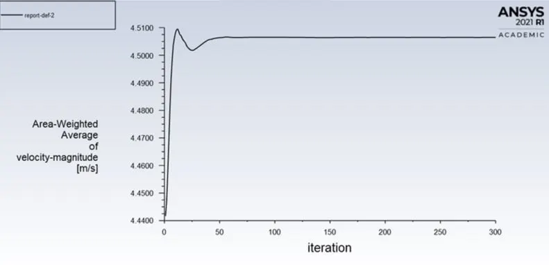
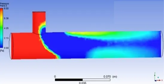
Velocity at outlet:

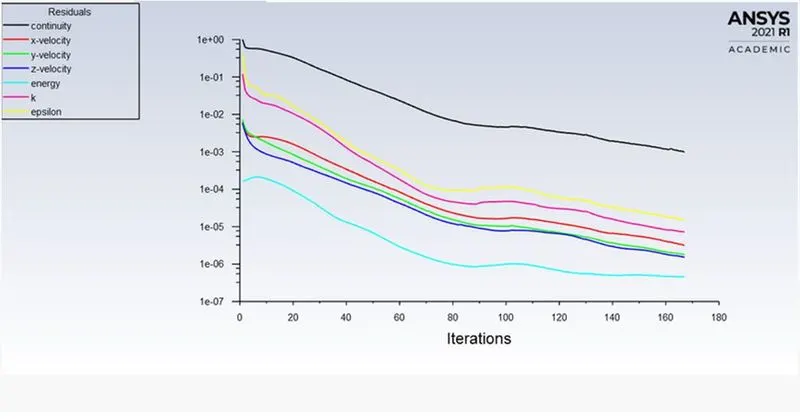
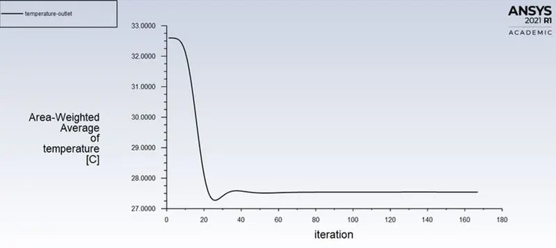
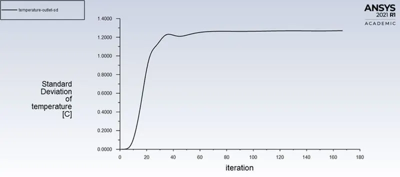
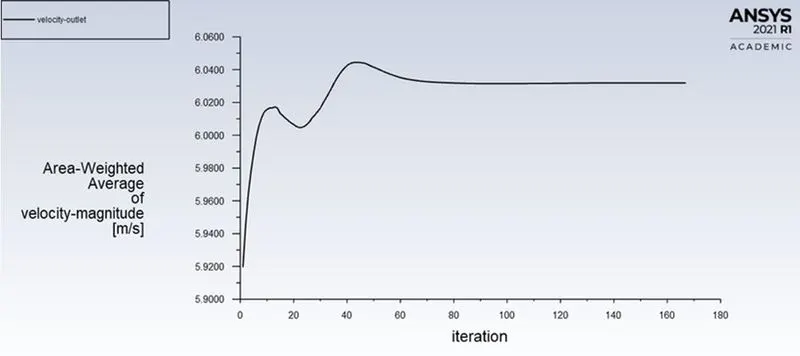
Short tee with momentum ratio 4:

Residuals:

Temperature at outlet:

Standard deviation of temperature at outlet:

Velocity at outlet:

Long tee momentum ratio 2:

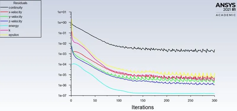
Residuals:

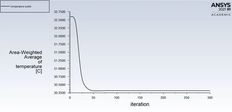
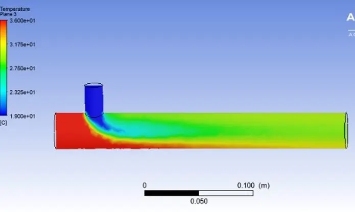
Temperature at outlet:

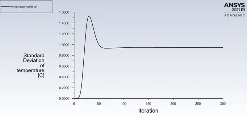
Standard deviation of temperature at outlet:

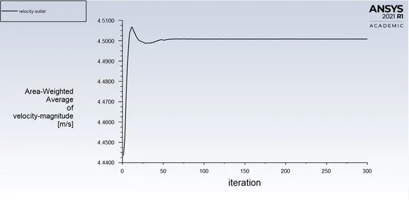
Velocity at outlet:

Long tee momentum ratio 4:

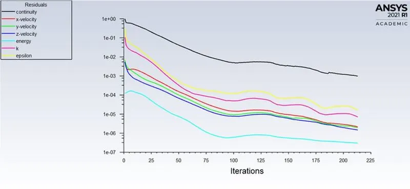
Residuals:

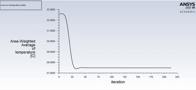
Temperature at outlet:

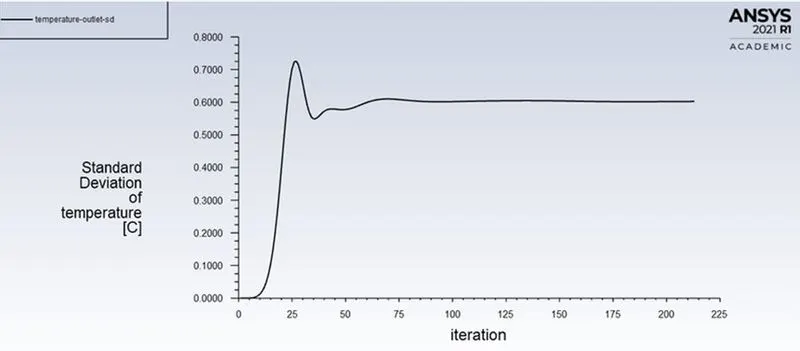
Standard deviation of temperature at outlet:

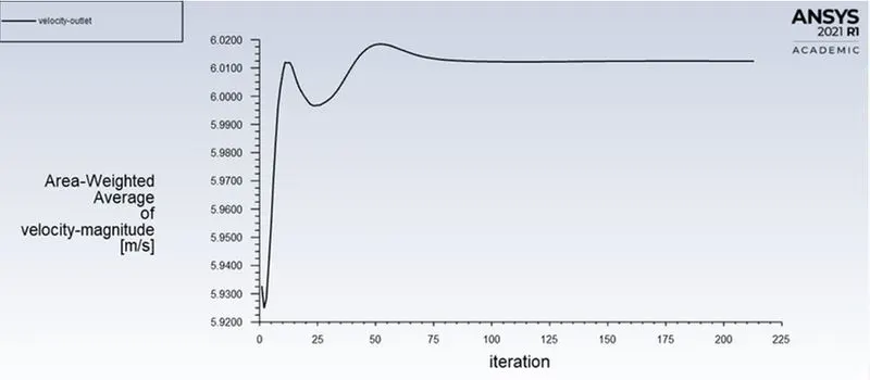
Velocity at outlet:

case 3:

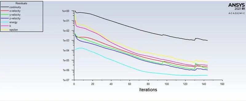
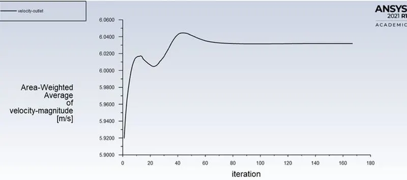
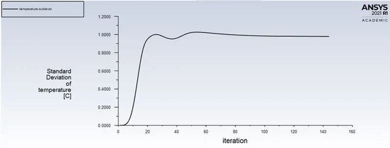
For 0.003

Residuals:

Velocity at outlet:

Standard deviation of temperature at outlet:

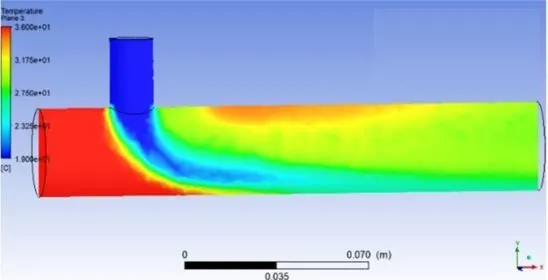
For 0.002

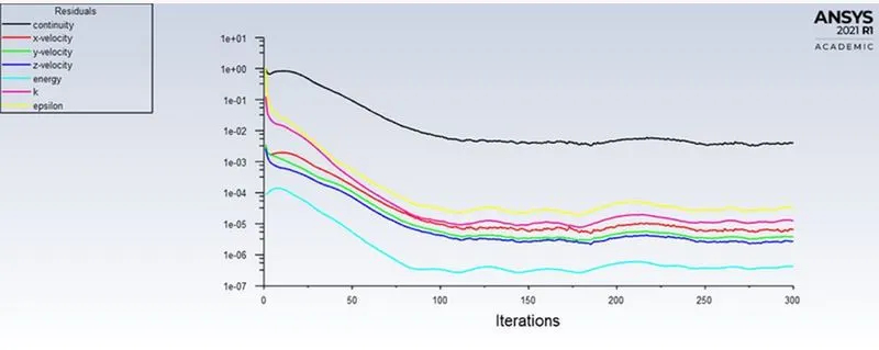
Residuals:

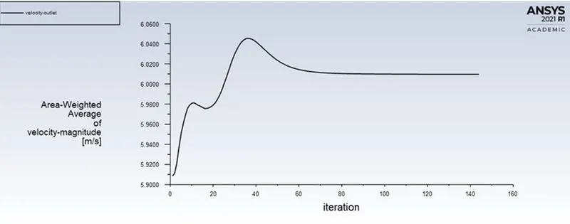
Velocity at outlet:

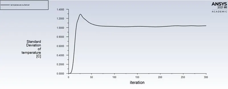
Standard deviation of temperature at outlet:

Conclusion

Outlet properties	Short Pipe(ratio 4)
	0.005	0.003	0.002
Outlet temperature	27.5 ˚C	27.5 ˚C	27.5 ˚C
Outlet velocity	6.03 m/s	6.03 m/s	6.03 m/s
Number of iteration	170	145	300
The standard deviation of temperature at the outlet	1.2 ˚C	0.98 ˚C	1 ˚C

As meshing size decreses the cell count increases and accuracy increases but the solver time increases so always do meshing according to the model and computer hardware.