Week 1- Mixing Tee

AIM: Calculate the temperature at the outlet.

INTRODUCTION: The function of the mixing tee challenge is the get the desire result at the outlet by changing its velocity of chilled air in room temperature.

THEORY:

SOLVING AND MODELLING APPROCH

ANSYS WORKFLOW:

Geometry: Construct the 2D or 3D geometry for the simulation.

Mesh: Meshing is the process cut the geometry into finite pieces.

Setup: In setup simulation is take place

SHORT TEE

GEOMETRY SETUP

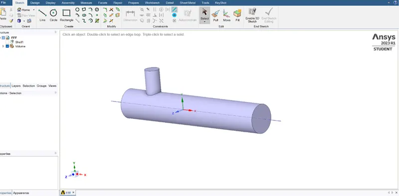
In this project we are performing fluid flow simulation through a pipe hence we used volume extraction option to extract the fluid flow from the geometry. Then the solid model is supressed for the physics from the fluid model to create the mesh.

MESH GENERATION

In meshing first, you have to give name Inlet_x, Inlet_y, and outlet for the identification.

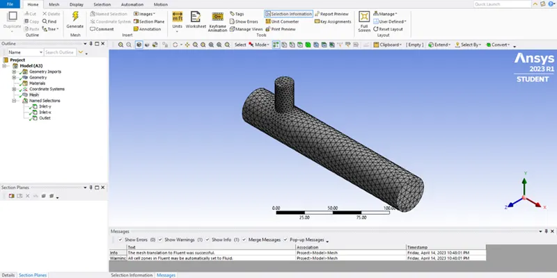
After generating mesh, the geometry converted into small piece and mesh quality also check.

SETUP AND SOLUTION

CASE:1

• Short mixing tee with a hot inlet velocity of 3m/s.
• Momentum ratio of 2,4.

CASE:1.1

• Short mixing tee with a hot inlet velocity of 3m/s
• Momentum ratio of 2.

SHORT TEE (MR=2 AND HOT INLET VELOCITY=3M/S)

SETUPS

K-EPSILON K-OMEGA

Solver type	Pressure based	Pressure based
Time	Steady	Steady
Viscous model	K-epsilon with wall function	k-omega with SST model
Material	Air	Air
Cell zones	· Inlet_x (velocity inlet) Velocity magnitude 3m/s Temperature -36˚c · Inlet_y (velocity inlet)	· Inlet_x (velocity inlet) Velocity magnitude 3m/s Temperature -36˚c · Inlet_y (velocity inlet)
Boundaries	· Velocity magnitude 6m/s Temperature -19˚c · Outlet (pressure outlet) Gauge pressure -0 Pa · Walls stationary walls	· Velocity magnitude 6m/s Temperature -19˚c · Outlet (pressure outlet) Gauge pressure -0 Pa · Walls stationary walls

From the above chart we can understand how fluid flow will go and what parameter we have to used here we used pressure-based solver because of density is constant hence the flow is incompressible.

RESULTS:

K-OMEGA MODEL:

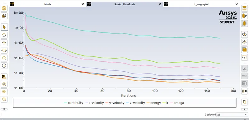
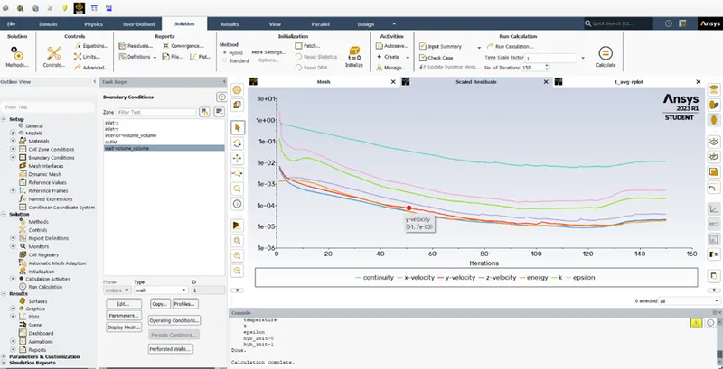
RESIDUAL PLOT:

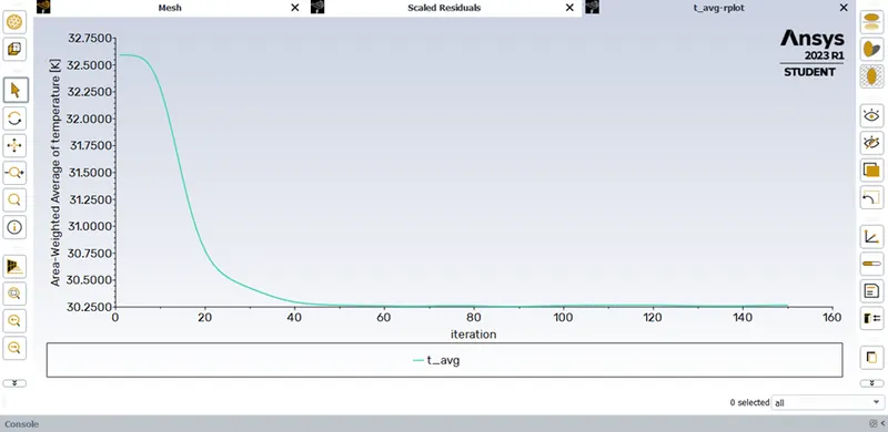
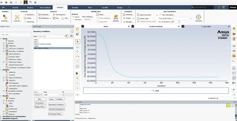
AREA WEIGHTED AVERAGE:

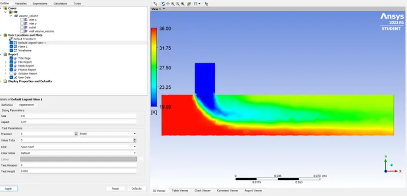
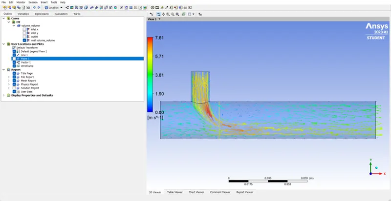
CONTOUR PLOT:

TEMPERATURE CONTOUR:

VELOCITY CONTOUR:

K-EPSILON MODEL:

RESIDUAL PLOT

AREA WEIGHTED AVERAGE

CONTOUR PLOT:

TEMPERATURE CONTOUR

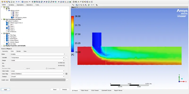
VELOCITY CONTOUR:

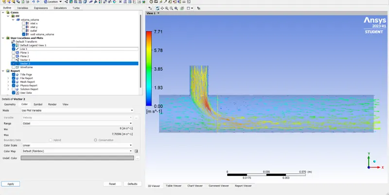
SUMMARY:

SHORT TEE(MR=2)

	K-EPSILON	K-OMEGA
Average outlet temperature[˚C]	32.592112	32.592112
No. of Iterations	150	150

CASE 1.2:

• Short mixing tee with hot inlet velocity of 3m/s
• Momentum ratio of 4

SHORT TEE (MR=4 AND HOT INLET VELOCITY =3 M/S)

SETUPS

	K-EPSILON	K-OMEGA
Solver type	Pressure based	Pressure based
Time	Steady	Steady
Viscous model	K-epsilon with wall function	K-omega SST model
Cell zones	· Inlet_x (velocity inlet) Velocity magnitude 3 m/s Temperature -36˚C · Inlet_y (velocity inlet)	· Inlet_x (velocity inlet) Velocity magnitude 3 m/s Temperature -36˚C · Inlet_y (velocity inlet)
Boundaries	Velocity magnitude 12 m/s Temperature -19˚C · Outlet (pressure outlet) Gauge pressure -0 Pa	Velocity magnitude 12 m/s Temperature -19˚C · Outlet (pressure outlet) Gauge pressure -0 Pa

In that hybrid scheme we are using for the initialization and the no. of iterations are setup to calculate.

RESULTS:

K-EPSILON MODEL:

RESIDUAL PLOT:

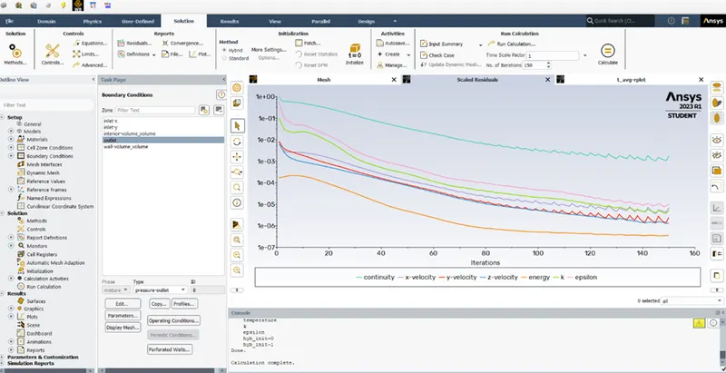
AREA WEIGHTED AVERAGE:

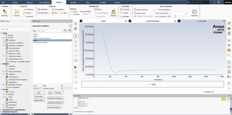
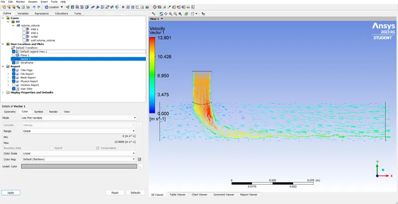
VELOCITY CONTOUR:

K-OMEGA MODEL:

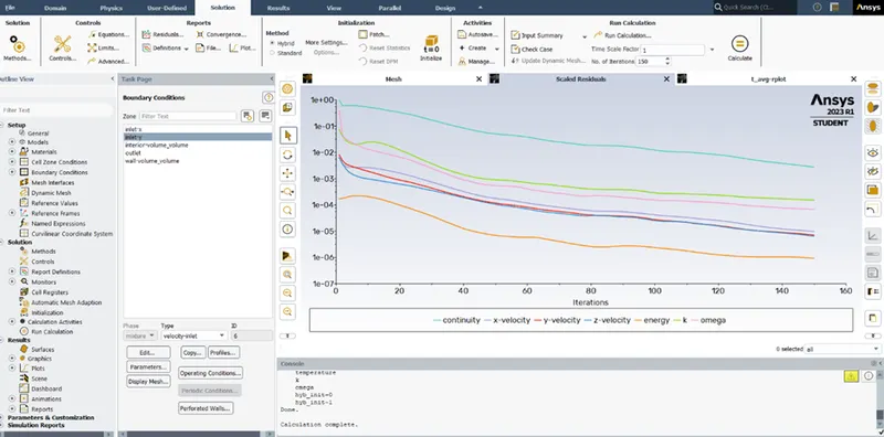
RESIDUAL PLOT:

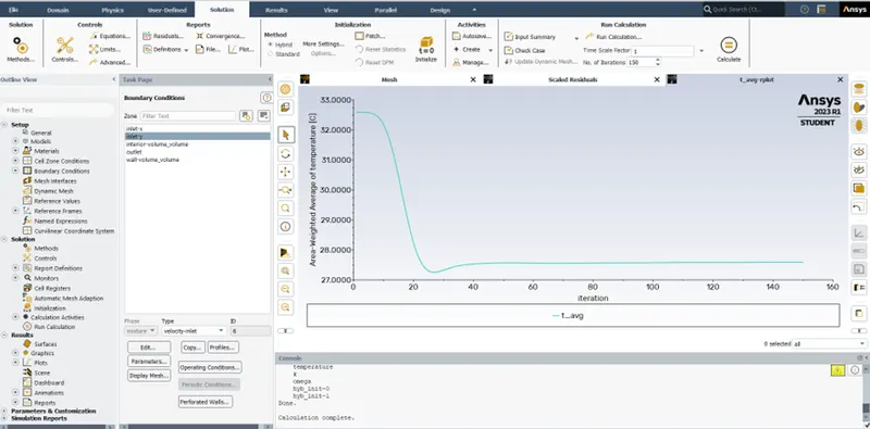
AREA WEIGHTED AVERAGE:

CONTOUR PLOT:

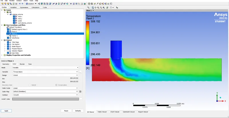
TEMPERATURE CONTOUR:

VELOCITY CONTOUR:

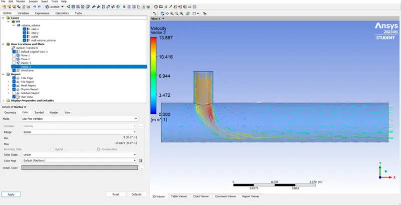
SUMMARY:

SHORT TEE (MR = 4)

	K-EPSILON	K-OMEGA
Average outlet temperature [˚C]	27.594759	27.591051
No.of iterations	150	150

ANALYTICAL SOLUTION:

MOMENTUM RATIO 2:

• Mass of hot fluid(m_h) = rho*a*V_h = 1.22*225*3 = 0.823 Kg/s
• Mass of cold fluid(m_c) = rho*a*V_c = 1.22*225*6 = 1.64 Kg/s
• Temperature of mixture (T_{mixture) = (}m_h*T_h+m_c*T_c)/(m_c+m_h)=24.68˚C

MOMENTUM RATIO 4:

• Mass of hot fluid(m_h) = rho*a*V_h = 1.22*225*3 = 0.823 Kg/s
• Mass of cold fluid(m_c) = rho*a*V_c = 1.22*225*12 = 3.294 Kg/s
• Temperature of mixture (T_{mixture) = (}m_h*T_h+m_c*T_c)/(m_c+m_h)=22.39˚C

CONCLUSION:

AVERAGE OUTLET TEMPERATURE

Comparing the both models with analytical solution we got the nearly same result.

ITERATION TO CONVERGE

No of iteration taken to converge is less for realisable k-epsilon model than k-omega SST model.

LONG TEE:

GEOMETRY SETUP:

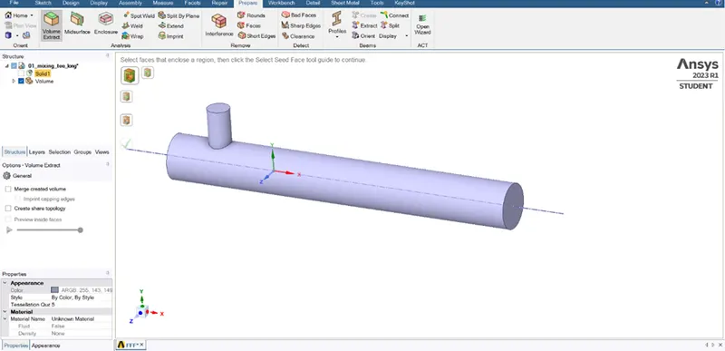
In this project we are performing fluid flow simulation through a pipe hence we used volume extraction option to extract the fluid flow from the geometry. Then the solid model is supressed for the physics from the fluid model to create the mesh.

MESH GENERATION

In meshing first, you have to give name Inlet_x, Inlet_y, and outlet for the identification.

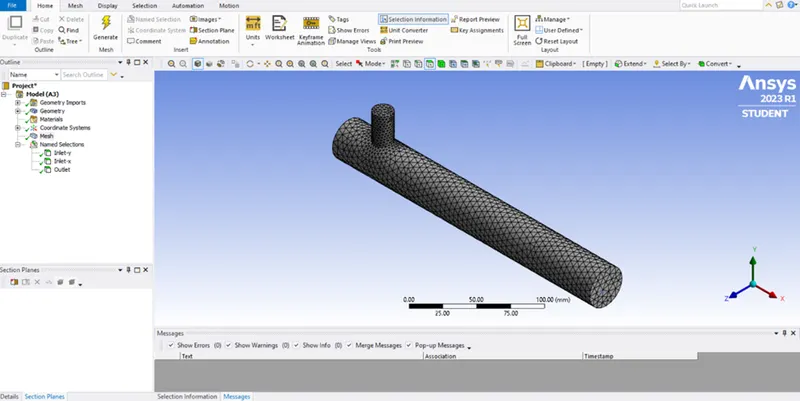
After generating mesh, the geometry converted into small piece and mesh quality also check.

SETUP AND SOLUTION

CASE:2

• Long mixing tee with a hot inlet velocity of 3m/s.
• Momentum ratio of 2,4.

CASE:2.1

• Long mixing tee with a hot inlet velocity of 3m/s
• Momentum ratio of 2.

LONG TEE (MR=2 AND HOT INLET VELOCITY=3M/S)

SETUPS

K-EPSILON

Solver type	Pressure based
Time	Steady
Viscous model	K-epsilon with wall function
Material	Air
Cell zones	· Inlet_x (velocity inlet) Velocity magnitude 3m/s Temperature -36˚c · Inlet_y (velocity inlet)
Boundaries	· Velocity magnitude 6m/s Temperature -19˚c · Outlet (pressure outlet) Gauge pressure -0 Pa · Walls stationary walls

From the above chart we can understand how fluid flow will go and what parameter we have to used here we used pressure-based solver because of density is constant hence the flow is incompressible.

RESULTS:

K-EPSIKON MODEL:

RESIDUAL PLOT:

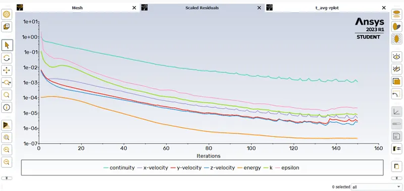
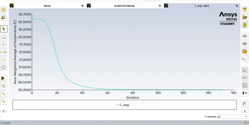
AREA WEIGHTED AVERAGE:

CONTOUR PLOT:

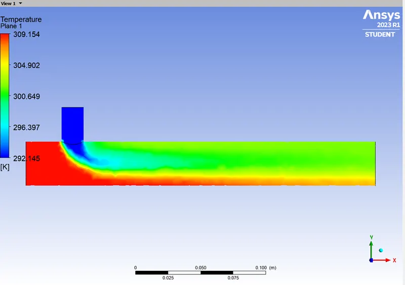
TEMPERATURE CONTOUR:

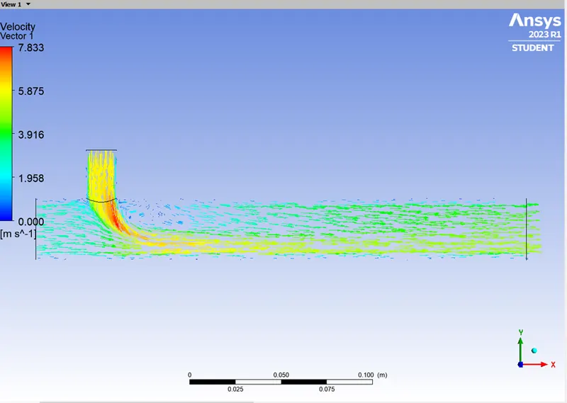
VELOCITY CONTOUR:

CASE 1.2:

• Long mixing tee with hot inlet velocity of 3m/s
• Momentum ratio of 4

SHORT TEE (MR=4 AND HOT INLET VELOCITY =3 M/S)

SETUPS

	K-EPSILON
Solver type	Pressure based
Time	Steady
Viscous model	K-epsilon with wall function
Cell zones	· Inlet_x (velocity inlet) Velocity magnitude 3 m/s Temperature -36˚C · Inlet_y (velocity inlet)
Boundaries	Velocity magnitude 12 m/s Temperature -19˚C · Outlet (pressure outlet) Gauge pressure -0 Pa

In that hybrid scheme we are using for the initialization and the no. of iterations are setup to calculate.

RESULTS:

K-EPSILON MODEL:

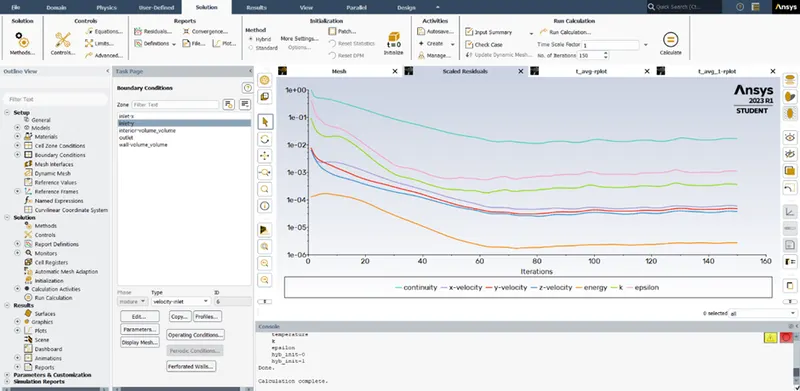
RESIDUAL PLOT:

AREA WEIGHTED AVERAGE:

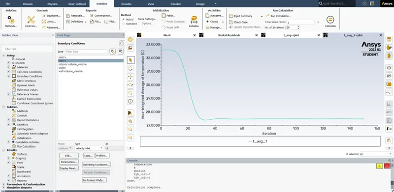
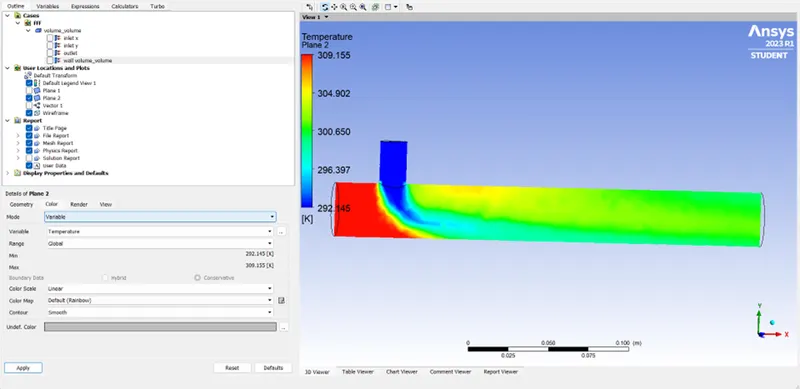
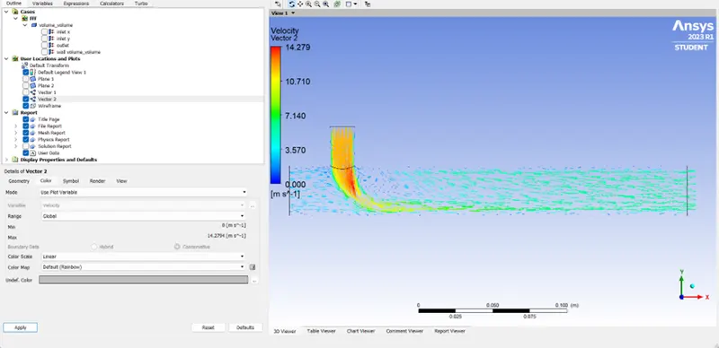
CONTOUR PLOT:

TEMPERATURE CONTOUR:

VELOCITY CONTOUR:

SUMMARY:

	LONG TEE(MR=2)	LONG TEE(MR=4)
Average outlet temperature (˚C)	30.260164	27.477953
No. of iterations	150	150

COMPARISON BETWEEN BOTH LONG AND SHORT TEE:

K-EPSILON MODEL:

GEOMETRY	MOMENTUM RATIO	CELL COUNT	AVERAGE TEMPERATURE (˚C)	NO. OF ITERATIONS
SHORT TEE	2	12692	32.592112	150
SHORT TEE	4	12692	32.592112	150
LONG TEE	2	15530	30.260164	150
LONG TEE	4	15530	27.477953	150

AVERAGE OUTLET TEMPRATURE:

Average outlet temperature in both cases nearly same.

CONCLUSION:

• Higher the momentum ratio, higher will be the efficiency of the mixing tee.
• Increasing the length of pipe the mixing will not get properly.