Week 1- Mixing Tee

Aim: To Simulate the Mixing Tee model under different cases and analyze the thermal variations.

• Case 1: mixing tee short model under momentum ratio of 2 and 4
• Case 2: mixing tee long model under momentum ratio of 2 and 4.

Note: Momentum ratio = ratio of the velocity of cold fluid to the velocity of hot fluid.

Introduction:

Computational fluid dynamics (CFD) is a branch of fluid mechanics that uses numerical analysis and algorithms to solve fluid flow situations. Computers are used to perform the calculations required to simulate the free-stream flow of the fluid, and the interaction of the fluid (liquids and gases) with surfaces defined by boundary conditions.

The Navier-Stokes (N-S) equation is the broadly applied mathematical model to examine changes in those properties during dynamic and/or thermal interactions.

• Conservation of Mass: Continuity Equation
• Conservation of Momentum: Newton’s Second Law
• Conservation of Energy: First Law of Thermodynamics or Energy Equation.

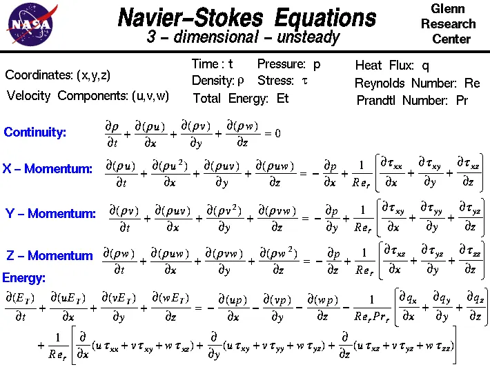
Discretization of the Navier–Stokes equations of fluid dynamics is a reformulation of the equations in such a way that they can be applied to computational fluid dynamics. Several methods of discretization can be applied:

• Finite volume method
• Finite elements method
• Finite difference method

Meshing: There are three types of grids: structured grids, unstructured grids, and heterogenous mesh (a combination of Structured and unstructured).

As smaller the mesh elements, accurate results are obtained. In the cost of time.

So, to mesh any object along with the size of an element other qualities are needed to check

1. Aspect ratio – the ratio of the cell’s longest length to the shortest length. As smaller, it is, the higher the quality.
2. Non-orthogonality – the angle between the vector connecting two adjacent cell centers and the normal of the faces shared by these cells. Ideal 0 and worst- 90.
3. Cell skewness: measures the deviation between the vertex angles of face pairs of a hexahedron. Ideal vertex angle of 90 degrees.
4. Volume ratio – maximum volume to the minimum volume of adjacent cells.

Modeling approach:

The model mixing tee is given, and boundary conditions were already mentioned.

1. Upload the model in Geometry
2. Create a volume extract in the prepared window in the space claim
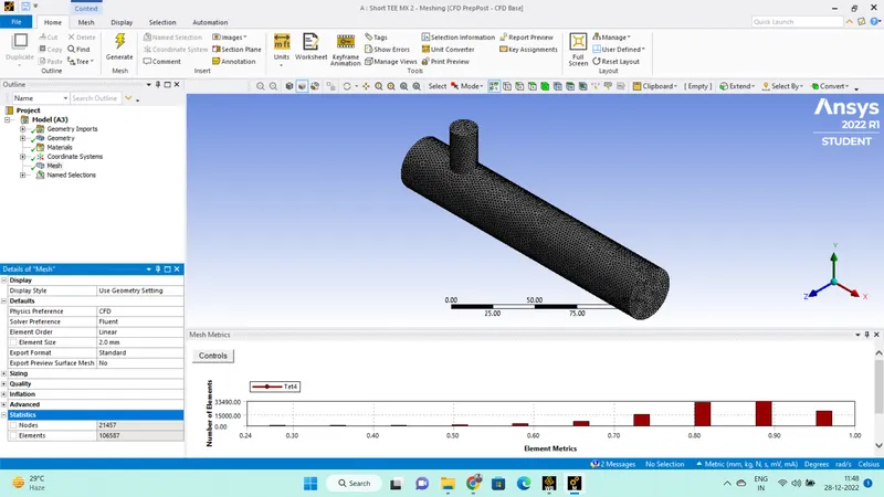
3. Create mesh, by using the sizing option we can adjust the element size. Also, create names such as inlet and outlet.

1. In Setup, in physics select the energy model, as we have the heat transfer.
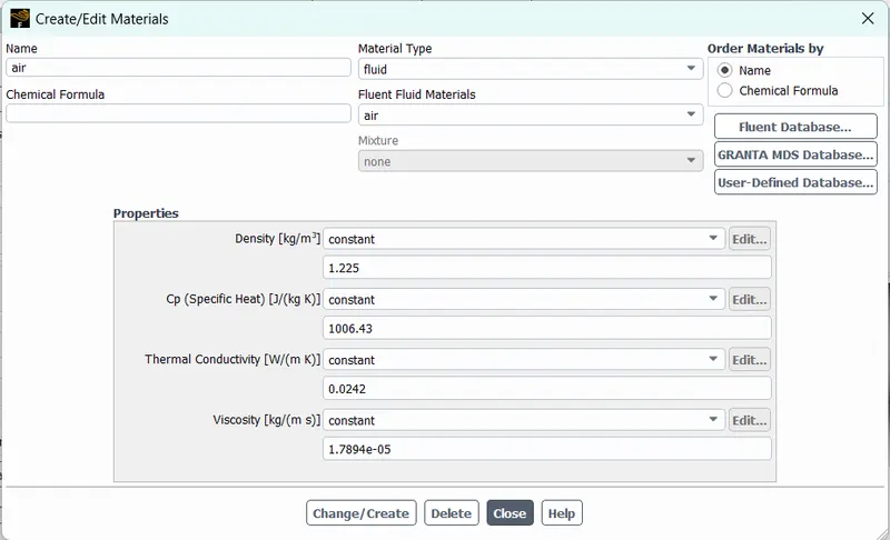
2. Give the material, for the current model let the fluid be air.
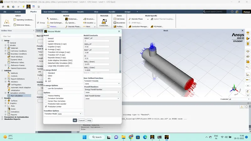
3. Under the viscous model, turbulent models have many different models, for the current model we select the K-epsilon à standard model.

Where K- turbulent kinetic energy

Epsilon – the rate of dissipation of kinetic energy.

7. K epsilon model is better when the region of interest flow is away from the wall boundaries and K-omega is better when the region of interest is close to the wall boundaries.

7. Define the boundary conditions, such as inlet velocities and outlet pressure = atmospheric pressure.

Input	Inlet X velocity (m/s) HOT	Inlet Y velocity (m/s) COLD	Outlet -pressure (Pa)	Momentum ratio
Short tee	3	6	101325	2
	3	12	101325	4
Long Tee	3	6	101325	2
	3	12	101325	4

Understanding the variation in results would be easy, if we take the same mesh size for all the cases.

9. Solution tab à definition à surface report and select different reports such as standard deviation and Average weighted average plots.
10. Select the initialization method as a hybrid. (Standard initialisation)
11. For the run calculations, let’s give 200 iterations
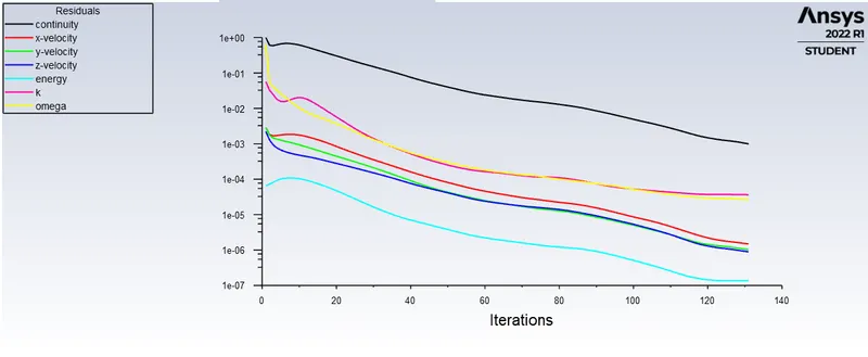
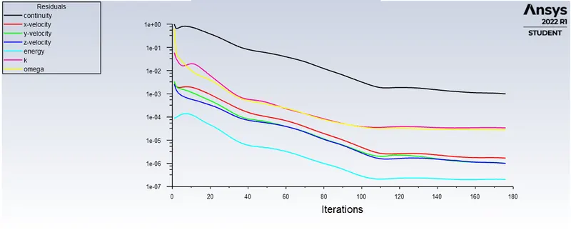
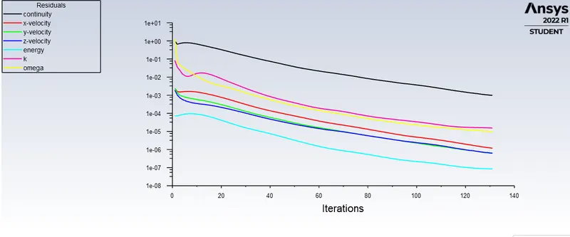
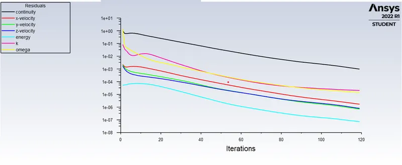
12. Iterations run until it gets converge. In the present case, the convergence is achieved below 200 iterations.
13. Even if we run beyond this, there won’t be much change in the results, just takes more time.
14. In the results tab, we can select the contour option to see the variations of different parameters along the space.

Eg: temperature gradient along and across the pipe, or Velocity contour along and across the plane or at any location of plane either in 3D or 2D view.

15. After the simulation to check the results select the type of report definition and select compute to get the output.
16. Under the report, à surface integral, whereby changing the field variables and computing the other parameters, such as mass flow rate, velocities, etc.
17. Now in the results, we can select different contours and charts to find the results and profiles.
18. If required, it can also generate streamlined plots and simulation animations in the results

Results:

	Momentum ration	Cell count	Average outlet temperature	No of iterations for convergence
Short Tee	2	106587	30.3620	131
	4	106587	27.601	176
Long Tee	2	140990	30.422	119
	4	140990	27.495	131

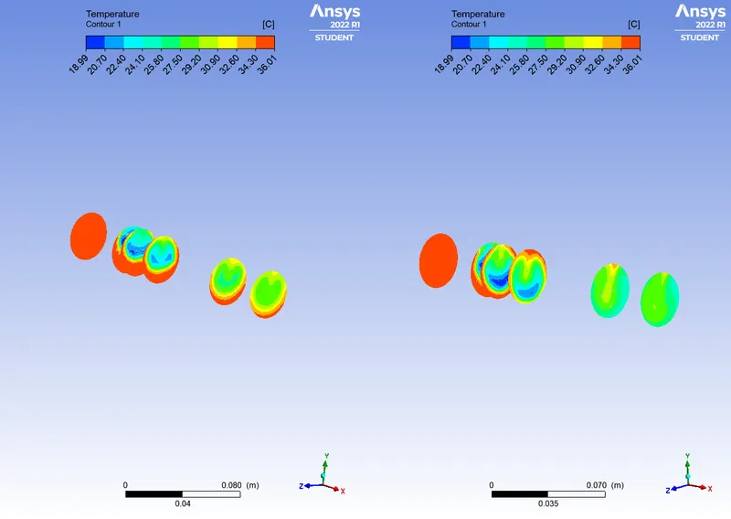
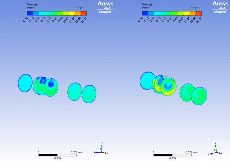
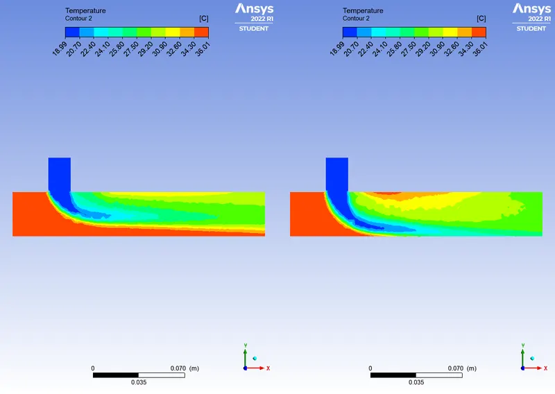
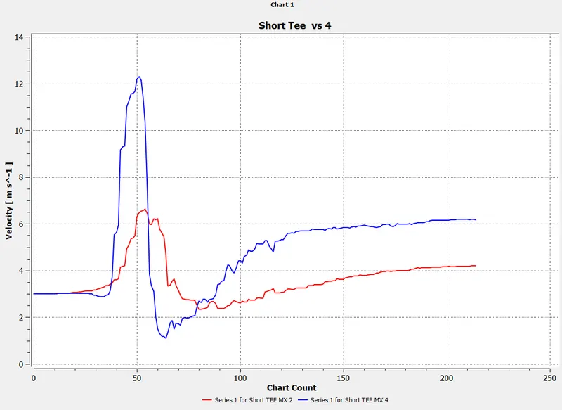
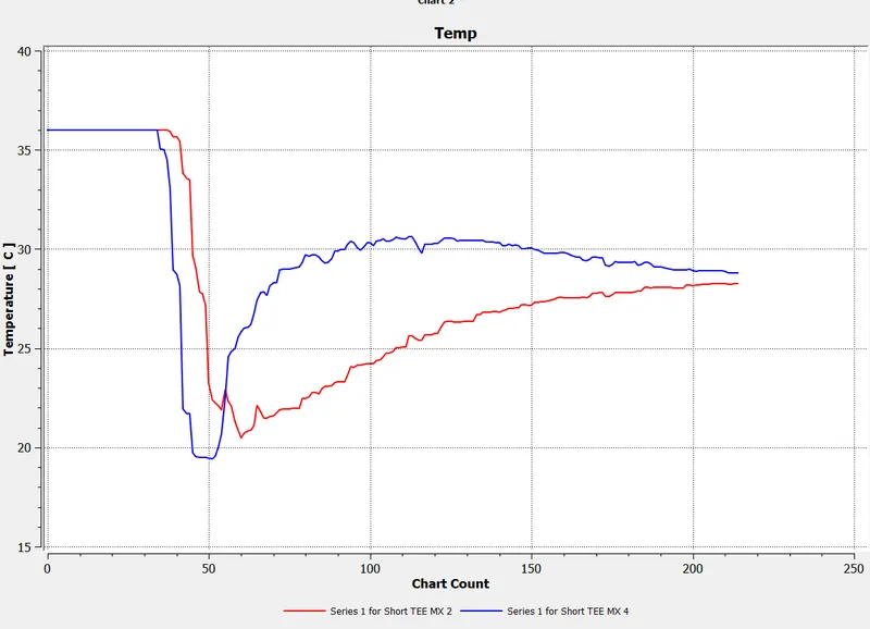
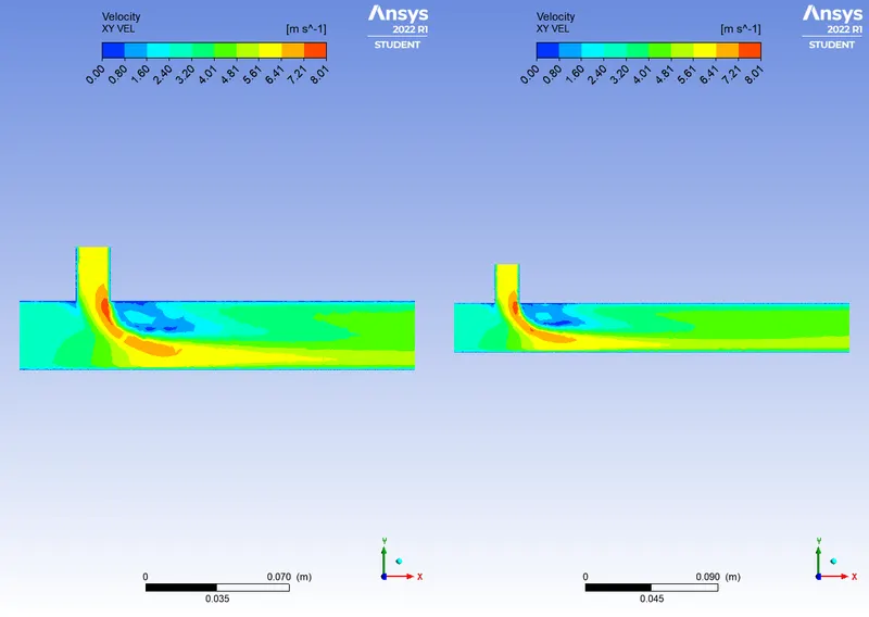
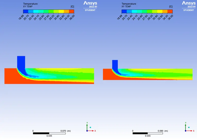
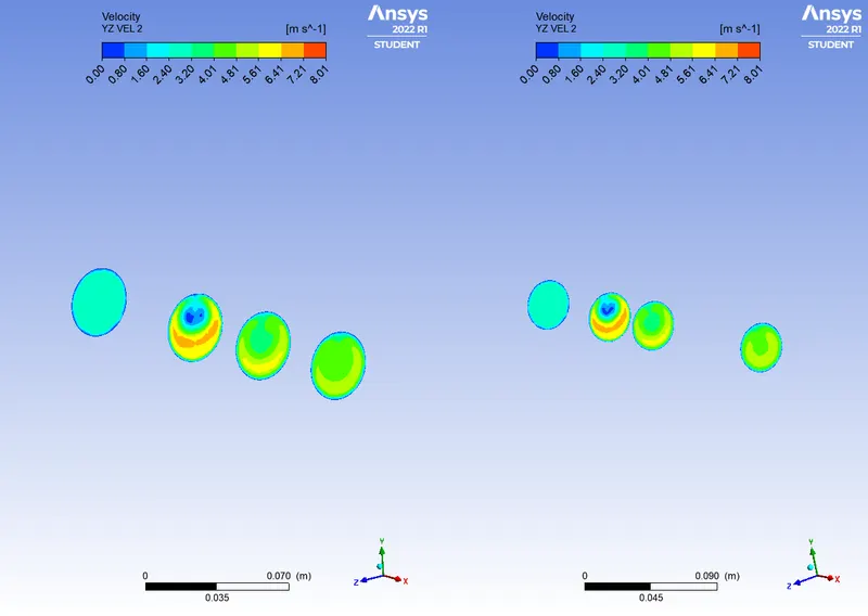
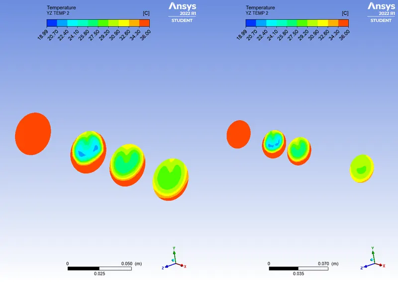
Comparing Momentum ratio of 2 and 4

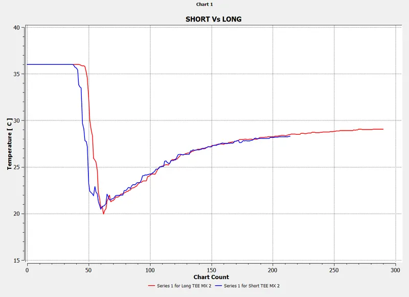
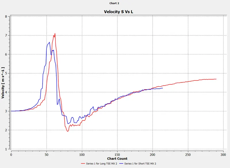
Comparing results of Long Vs Short Tee

Mesh independent study

This can be performed by finding the variations in the temperature due to different mesh sizes, the smaller the mesh more accurate the results. After some mesh size, the results converge. that means the value of temperature won't change even if the mesh size is reduced. this mesh size is called optimal or critical mesh size

Convergence plots

Conclusions

From the results of graphs and 3D images we can conclude the effect of length and mixing ratio on temperature and velocity

In a comparison of the Mixing ratio of 2 Vs 4

1. With a higher mixing ratio, exit velocities are more.
2. The distribution or diffusion of cold fluid entering from a small inlet is even in a higher mixing ratio and temperature distributions are also almost equal throughout the cross-section at the outlet position
3. No of iteration taken to solve is more for higher momentum ratio

Better mixing of fluids will be better for higher mixing ratios

In comparison to Long and Short

1. Long tee and short tee both have similar heat transfer or temperatures at the center.
2. But the velocity curves are also more similar in both cases.

So, there is not much effect on the length of the pipe after mixing. But the outlet temperatures are more sensitive to the Momentum ratio