Week 1- Mixing Tee

Introduction:

In fluid dynamics, turbulence or turbulent flow is fluid motion characterized by chaotic changes in pressure and flow velocity. It is in contrast to a laminar flow, which occurs when a fluid flows in parallel layers, with no disruption between those layers.

Mixing tee is basically mixing the fluid in the model which looks like T shape structure. Here the mixing is between the hot air with the cold air. Here in a mixing Tee Model we use two types of fluid passes through two different inlets and at different temperatures flows through these ports. This analysis is mainly to see how these flows and different temperatures acting in the mixing tee model. We use here two different types mesh study to see how the fluctuations in the flow for two different types of flow. This is generally Air condition systems seen in our homes, offices, shops, internet station etc.

For example in summer we need a cooled air inside the room. This can be solved by using air cooler. The working principle behind this is mixing the atmospheric cleaned air and the cooled air generated by the air cooler.

The hot air coming from the atmosphere is usually of 30-45⁰c and the cooled air generated by the air cooler is from 0-20⁰c. When we mix these two types of air the output air should be around room temperature between 20-25⁰c. In order to make this possible the model should be such that it should mix properly before it delivers. To do this the model is created in the respected software. Here we are using solid works to create this model.

We are using Ansys fluent for the CFD simulation of the turbulence mixing model. We are considering some models to define the appropriate values of the mixing air. In the Ansys fluent mesh parameter and solving the problem by CFD simulation and giving a detailed description of the result, we can use these data to compare with the experimental data.

Aim

1. Velocity and temperature contour plots on the cut planes along and across the pipe.
2. Velocity and temperature line plots along and across the length of the pipe.
3. Perform Mesh independent study for any one case.
4. Discuss the effect of length and momentum ratio on results.

There are mainly 3 steps to solve in order to get these results i.e.

1. Pre processing
2. Solving
3. Post Processing

Pre processing approach:

In this approach we do designing the geometry, for the required simulation. Depending upon the geometry we should clean up the geometry and extract the volume from the geometry, providing the names for the geometry, discretize the entire domain into tiny volumes, assigning initial and final boundary conditions.

Modelling Approach:

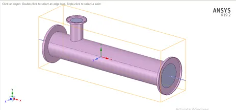
Here we are designed two types of model, which is with short pipe length and long length of pipe for mixing both types of air. The diameter of the pipe is fixed and length of the pipe is varied. The diameter we took here is 35mm and for short pipe length here i took around 200mm and for long pipe the length of the pipe is 275mm.

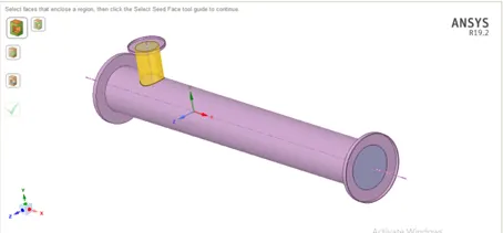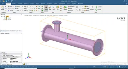
The model is edited in the space claim to obtain only the flow in Ansys Workbench geometry tab; this is done by extract the volume from the model- and suppresses the solid model as per the required cases

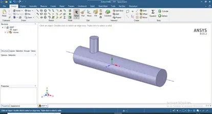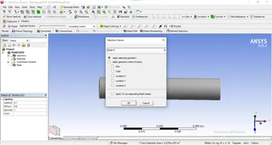
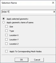
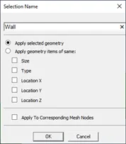
Suppressing the model is because the fluid analysis will not take part on the solid model it only show the flow properties within the solid model. The next part of analysis is meshing the model. Here as soon as we open the mesh tab the geometry will loaded, now by using face selection tab- and rename the model like hot inlet, cold inlet, outlet & walls. After renaming, give the mesh quality and size based on this mesh the fluid flow analysis can be obtained.

Case 1:

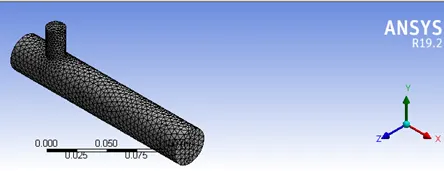Fig a

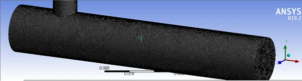Fig b

Short pipe mesh (Fig a=5mm, Fig b=1mm)

Case 2:

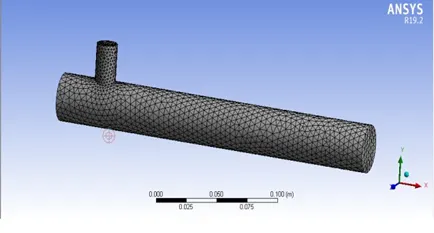Fig a

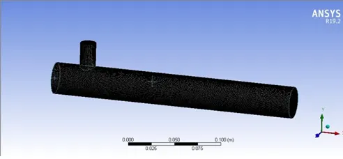Fig b

Long pipe mesh (Fig a=5mm, Fig b=1mm)

Solution:

In order to solve the system of the partial differential equation we get we need to provide the right initial preliminary parameters should be given to see how the flow varies between the types of pipes. Boundary conditions like flow velocity, energy, turbulence, material, number of iterations, etc.

Boundary conditions:

Solver	Steady state, Pressure Based
Mesh	Tria Element type
Turbulence(viscosity)	K-Ɛ, K- ω
Material	Fluid(Air)
Cold Inlet velocity	6 m/s, 12 m/s
Hot Inlet Velocity	3 m/s
Cold Inlet Temperature	190C
Hot Inlet Temperature	360C
Outlet velocity	Atmospheric Pressure(atm)

Steady state solver means the fluid flow does not change over time and transient solver is the flow change over time.

Pressure based solver is used for low speed flows and Mach number below 0.3 and for incompressible flow and density based solver is for high speed flows and compressible flow.

Computer cannot solve partial differential equation, hence these partial differential equations are converted into a form where the system can solve this type of equation is known as Discretization. Partial differential equations are in continuous form. At any x,y z point the density, velocity and temperature are solved by means of discrete points, shapes or volumes

Discretization is the process through which we can transform continuous variables, Models or functions into a discrete form. There are mainly 3 different types of Discretization namely

1. Finite Element Method
2. Finite Difference Method

• Finite Volume Method

Finite element is discretize entire domain into equal number of 2d elements

Finite difference is discretize entire space into points

Finite element is discretize entire domain into equal number of small volumes

These 3 types can solve any types of partial differential equations.

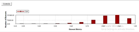
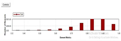
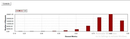
Mesh is nothing but discritizing or cutting or dividing the model into very small tiny spaces where the Navier stroke equation apply and makes the solution and by doing so for all the discritised spaces it will provide us the final result by plotting the required graphs along the pipe location. Here the mesh can be dived into two type’s i.e. coarse and fine mesh. The coarse mesh is known as the higher mesh size and fine mesh is known as lower mesh size. Here i took coarse mesh as 5mm, and fine mesh as 1mm. better the mesh size and quality the improvement in the flow properties can be seen

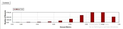Short Pipe 5mm	Short Pipe 1mm
Long Pipe 5mm	Long Pipe 1mm

In CFD to get more information about the simulation Turbulence should be given. The different type of turbulence models are

• Reynolds average Navier stroke (RANS)
• Large Eddy Simulation (LES)
• Direct Numerical simulation (DNS)

Majority of engineering simulation is RANS based. RANS based simulation are less accurate than LES based simulation and LES based simulation is less accurate than DNS based simulation. But in terms of speed RANS based simulation are much faster than LES based simulation.

In RANS based simulation generally of two types

• K-Ɛ
• K- ω

K-epsilon model is ideal for predicting the flow behaviour away from the wall and

K- Omega model is well suited for simulating flow in viscous sub layer.

The Inlet velocity is considered by means by means of Momentum Ratio. Momentum ratio is the ratio between the velocity at the cold inlet to the velocity at the hot inlet. As given for the solution for momentum ratio for 2& 4 and the hot inlet velocity given here is 3m/s. Therefore the inlet velocity is 6 m/s and 12 m/s.

For the analysis purpose by keeping the iterations constant at 400, we take two types of cases namely

Case1(Short Pipe)	Mesh- coarse-5mm & Fine -1mm Hot Inlet Velocity-3m/s Cold inlet velocity -6m/s and 12 m/s Turbulence Model- K-Ɛ and K- ω Iterations-400
Case2(Long Pipe)	Mesh- coarse-5mm & Fine -1mm Hot Inlet Velocity-3m/s Cold inlet velocity -6m/s and 12 m/s Turbulence Model- K-Ɛ and K- ω Iterations-400

	Case1		Case2
	Short 5 mm	Short 1 mm	Long 5 mm	Long 1 mm
Elements	14410	579963	18180	769722
Nodes	3166	111131	4017	147695

It can be seen that from the above table when compare with 5mm and 1mm mesh element size, for the higher mesh size the elements and nodes are very less, but for the lower mesh size the elements and nodes are high.

Below are the set of results obtained from the analysis for K-Ɛ and K- ω

K-Ɛ Model

Case1(Coarse Mesh)5mm-6m/s	Case1(Fine Mesh)1mm-6m/s
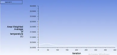Area Weighted Avg Temp-30.190C	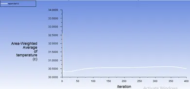Area Weighted Avg Temp-30.520C
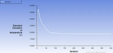Standard deviation temp-1.760C	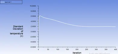Standard deviation temp-1.880C

Case1(Coarse Mesh)5mm-12m/s		Case1(Coarse Mesh)1mm-12m/s
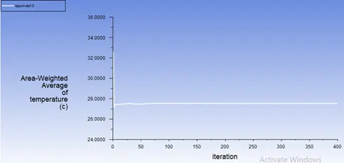Area Weighted Avg Temp-27.530C	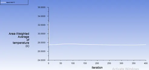	Area Weighted Avg Temp-27.530C
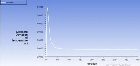Standard deviation temp-0.890C	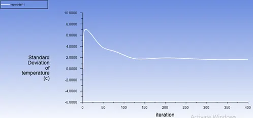Standard deviation temp-1.610C

In the similar manner below results are obtained by running the simulation for different boundary Mesh size, velocity & Turbulence model.

	Velocity	6 m/s		12 m/s		6 m/s			12 m/s
	Turbulence/Mesh	K-Ɛ				K- ω
Case 1 Short Pipe	0.005(5mm)	AWAT	30.190C	AWAT	27.530C		AWAT	30.20	AWAT	27.540C
		STDT	1.760C	STDT	0.890C		STDT	2.200C	STDT	1.000C
	0.001(1mm)	AWAT	30.500C	AWAT	27.530C		AWAT	30.450C	AWAT	27.650C
		STDT	1.880C	STDT	1.610C		STDT	2.600C	STDT	2.050C
Case 2 Long Pipe	0.005(5mm)	AWAT	30.320C	AWAT	27.480C		AWAT	30.340C	AWAT	27.480C
		STDT	0.680C	STDT	0.780C		STDT	1.140C	STDT	0.790C
	0.001(1mm)	AWAT	30.570C	AWAT	27.410C		AWAT	30.630C	AWAT	27.600C
		STDT	1.290C	STDT	0.950C		STDT	1.840C	STDT	1.140C
	AWAT-Area Weighted Average Temperature(0C)
	STDT-Standard Deviation Temperature(0C)

Post processing approach:

Finally once the simulation is done we should analyze the result which is the most important part of any analysis. The initial conditions given should be such that better results should be obtained from these simulations. This must be both qualitative and quantitative.

Mesh independent study:

Temperature Contour:

Case1-K-Ɛ-6m/s	Case1-K- ω-6m/s
Case1-K-Ɛ-12m/s	Case1-K- ω-12/s
Case2-K-Ɛ-6m/s	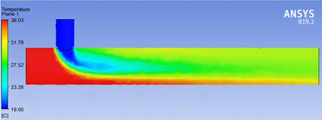	Case2-K-ω-6m/s
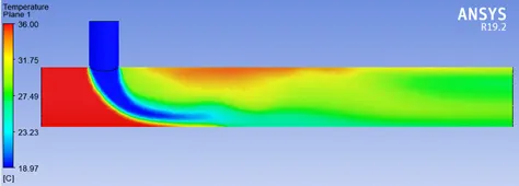Case2-K-Ɛ-12m/s	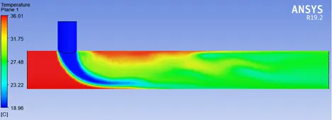	Case2-K-ω-12m/s

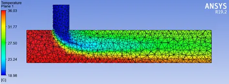Case1-K-Ɛ-6m/s	Case1-K- ω-6m/s
Case1-K-Ɛ-12m/s	Case1-K- ω-12/s
Case2-K-Ɛ-6m/s		Case2-K-ω-6m/s
Case2-K-Ɛ-12m/s		Case2-K-ω-12m/s

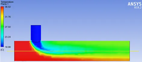
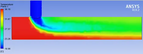
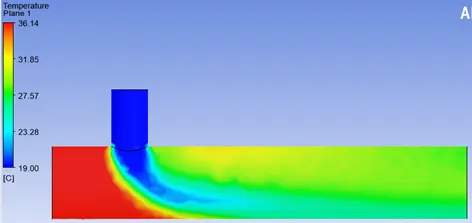
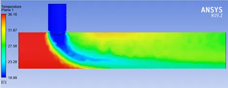
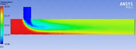
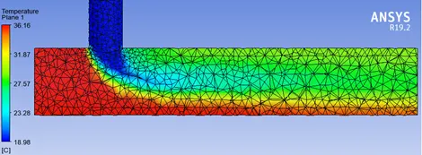
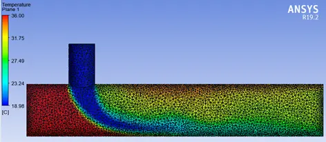
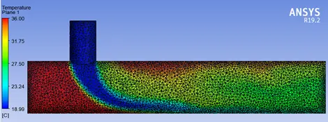
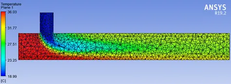
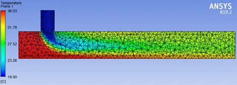
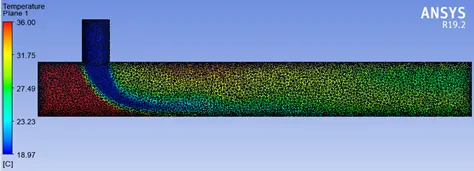
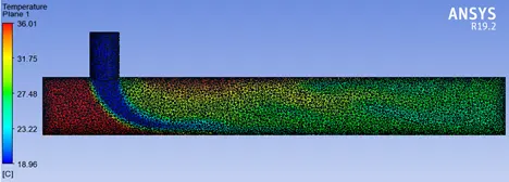
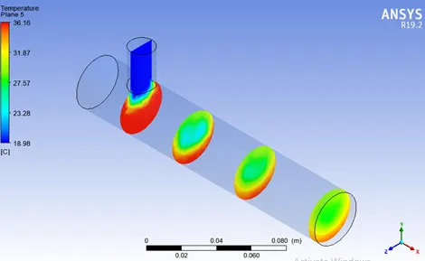
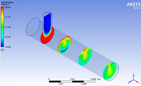
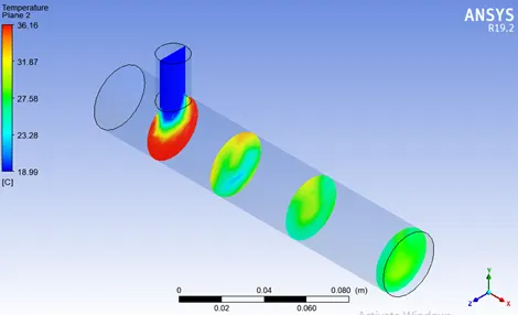
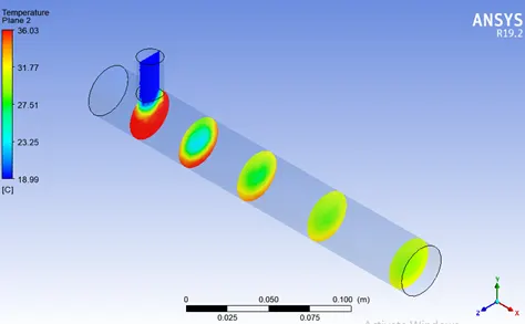
In the Coarse mesh the mixing of the temperature variation is not clearly defined but in the fine mesh, we can see the temperature lines are clearly defined. The fluctuation of the temperature after mixing is more in the coarse mesh model but in the fine mesh, it reduces.

	Velocity	6 m/s		12 m/s		6 m/s			12 m/s
	Turbulence/Mesh	K-Ɛ				K- ω
Case 1 Short Pipe	0.005(5mm)	Max Temp	31.76	Max Temp	27.57		Max Temp	36.16	Max Temp	27.58
		Min Temp	27.50	Min Temp	23.28		Min Temp	27.57	Min Temp	23.28
	0.001(1mm)	Max Temp	31.75	Max Temp	31.75		Max Temp	36	Max Temp	31.75
		Min Temp	27.50	Min Temp	23.24		Min Temp	23.24	Min Temp	27.50
Case 2 Long Pipe	0.005(5mm)	Max Temp	31.77	Max Temp	27.51		Max Temp	31.78	Max Temp	31.77
		Min Temp	27.51	Min Temp	23.25		Min Temp	27.52	Min Temp	27.50
	0.001(1mm)	Max Temp	31.75	Max Temp	31.75		Max Temp	31.74	Max Temp	27.48
		Min Temp	27.49	Min Temp	27.49		Min Temp	27.49	Min Temp	23.22

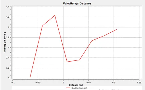
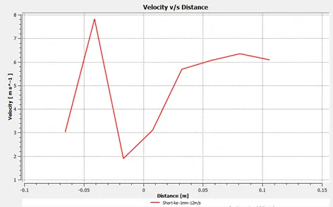
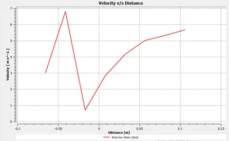
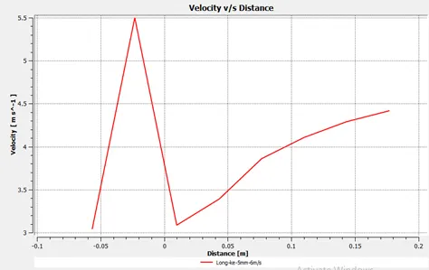
There is a sudden rise is due to the high velocity fluid enters to the pipe at this length of pipe and as move forward the mixing of fluids with different velocity and gets try to balance as length of pipe increases.

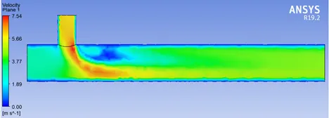
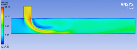
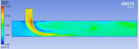
Velocity Contour:

Case1-K-Ɛ-6m/s	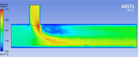Case1-K- ω-6m/s
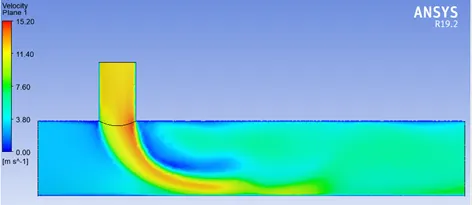Case1-K-Ɛ-12m/s	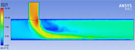Case1-K- ω-12/s
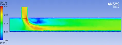Case2-K-Ɛ-6m/s		Case2-K-ω-6m/s
Case2-K-Ɛ-12m/s		Case2-K-ω-12m/s

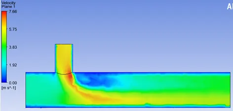
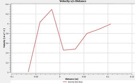
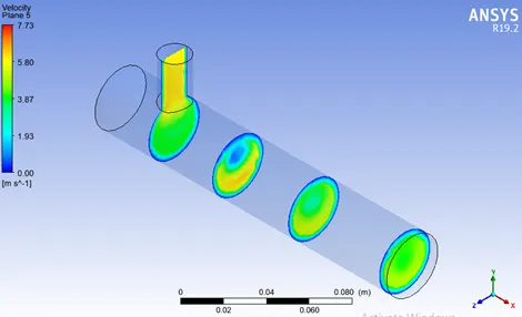
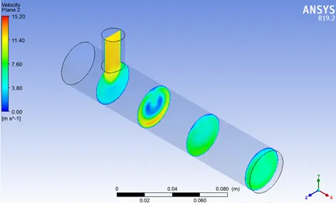
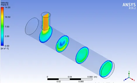
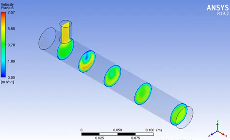
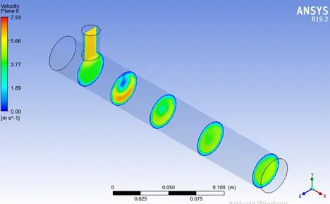
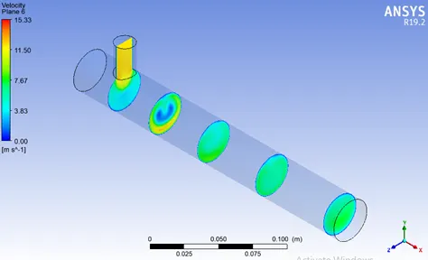
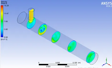
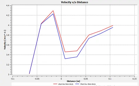
Due to high velocity fluid mixed with low velocity fluid there is sudden change in velocity. As soon as enters near the T section there is a sudden velocity drop this is because both low velocity high temperature from hot inlet mixes with High velocity-Low temperature mix together creates a turbulence and hence the color of the velocity changes from where blue color mixes with green color.

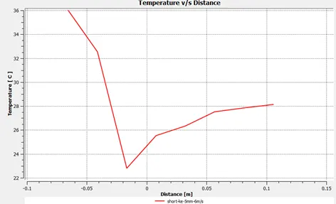
Temperature profile:

Case1-K-Ɛ-6m/s	Case1-K- ω-6m/s
Case1-K-Ɛ-12m/s	Case1-K- ω-12/s
Case2-K-Ɛ-6m/s		Case2-K-ω-6m/s
Case2-K-Ɛ-12m/s		Case2-K-ω-12m/s

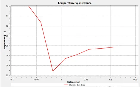
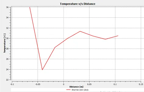
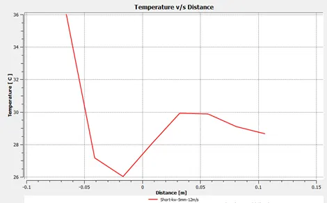
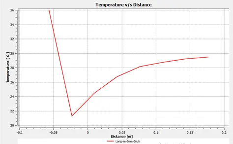
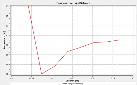
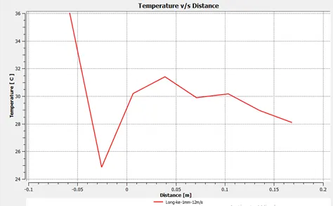
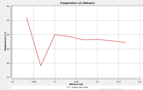
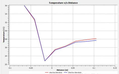
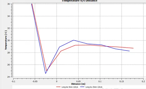
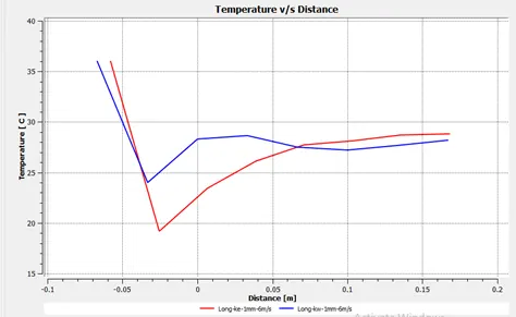
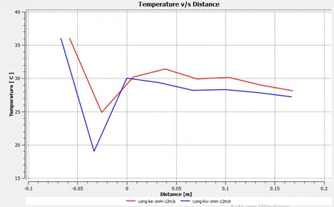
There is a sudden dip and rise happen when hot ait mixed with cold air and as it moves further due to the turbulence the flow get steady state along the pipe. But if the pipe length is increases there is nothing drastic changes happen but the velocity get decresed and temperature get hotter when the length of the pipe increased.

Velocity profile:

Case1-K-Ɛ-6m/s	Case1-K- ω-6m/s
Case1-K-Ɛ-12m/s	Case1-K- ω-12/s
Case2-K-Ɛ-6m/s	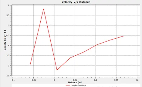	Case2-K-ω-6m/s
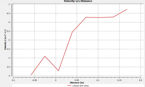Case2-K-Ɛ-12m/s	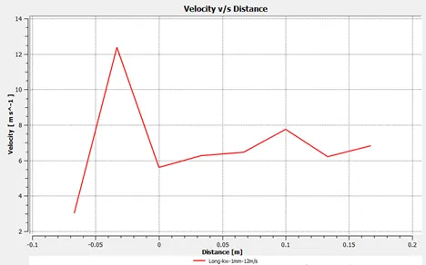	Case2-K-ω-12m/s

Temperature cut across the pipe

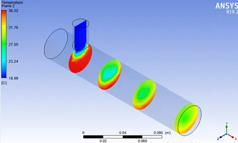Case1-K-Ɛ-6m/s	Case1-K- ω-6m/s
Case1-K-Ɛ-12m/s	Case1-K- ω-12/s
Case2-K-Ɛ-6m/s	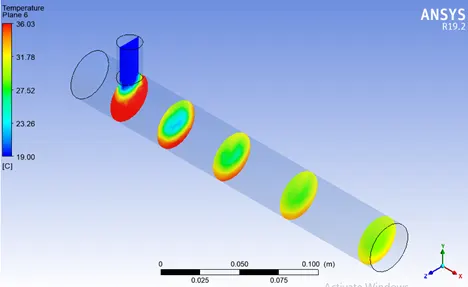	Case2-K-ω-6m/s
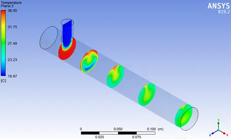Case2-K-Ɛ-12m/s	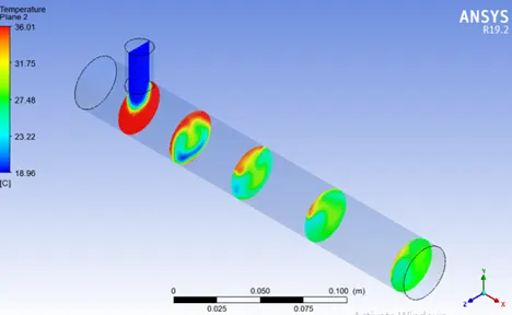	Case2-K-ω-12m/s

Velocity cut across the pipe

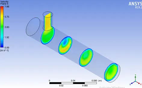Case1-K-Ɛ-6m/s	Case1-K- ω-6m/s
Case1-K-Ɛ-12m/s	Case1-K- ω-12/s
Case2-K-Ɛ-6m/s		Case2-K-ω-6m/s
Case2-K-Ɛ-12m/s		Case2-K-ω-12m/s

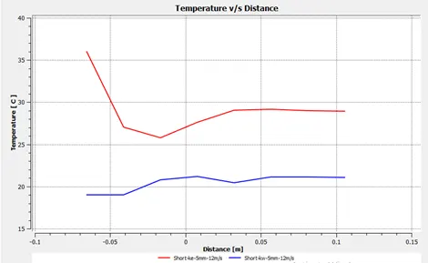
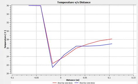
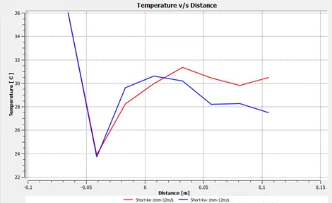
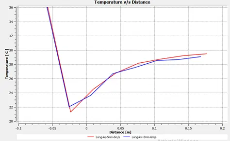
Temperature Comparison between Coarse and Fine Mesh for different velocity

Case1-K-Ɛ& K-ω -6m/s	Case1- K-Ɛ& K-ω-12m/s
Case1-K-Ɛ& K-ω -6m/s	Case1-K-Ɛ& K-ω -12m/s
Case2-K-Ɛ& K-ω -6m/s		Case2-K-Ɛ& K-ω -6m/s
Case2-K-Ɛ& K-ω -6m/s		Case2-K-Ɛ& K-ω -6m/s

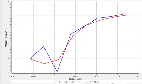
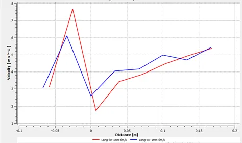
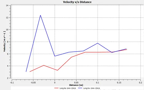
Velocity Comparison between Coarse and Fine Mesh for different velocity

Case1-K-Ɛ& K-ω -6m/s	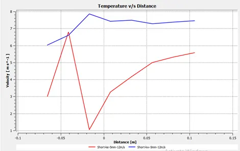Case1- K-Ɛ& K-ω-12m/s
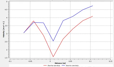Case1-K-Ɛ& K-ω -6m/s	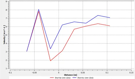Case1-K-Ɛ& K-ω -12m/s
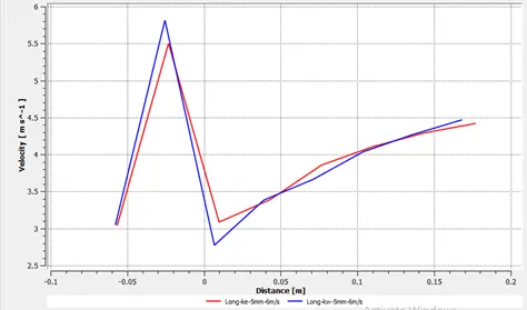Case2-K-Ɛ& K-ω -6m/s		Case2-K-Ɛ& K-ω -6m/s
Case2-K-Ɛ& K-ω -6m/s		Case2-K-Ɛ& K-ω -6m/s

As length of pipe increases there is no change in temp line plot, the plots gets coincide.

Results & Conclusion

From the above analysis below are the some results listed here.

Mesh: In Mesh parameter the model can be meshed by two types i.e. coarse or Fine. In coarse mesh the mesh elements and nodes are very less where as in Fine mesh these elements and nodes are very which will help to capture the results very accurately. But as we go increase the mesh size the results we get is much slower than coarse mesh because the Navier stoke equations should be apply for the high number of Nodes and Elements.

Area weighted Average Temperature and Standard Deviation Temperature:

When compare coarse and fine mesh the area weighted temperature increases and standard deviation temperature for fine mesh, but if the cold inlet velocity increase it decreases in both K-Ɛ& K-ω models.

Temperature and velocity contour along the Pipe:

For the low velocity and coarse mesh the hot inlet temperature moves up to the end of the pipe. But for higher cold inlet velocity increases the temperature mixes properly due to the turbulence effect and the out temperature varies independently.

The minimum outlet temperature obtained at the outlet in coarse mesh with low and high velocity is near 23.28⁰C, and in fine mesh it not much decreases it is around 23.24. as the length of the pipe increases also the temperature didn’t dip instead the temperature rises. And hence its conclude that fine mesh with shorter pipe length provides the required room temperature.