Week 1- Mixing Tee

AIM:

• To set up steady-state simulations to compare the mixing effectiveness when hot inlet temperature is 36⁰C & the Cold inlet is at 19⁰C using k-epsilon and k-omega SST model for the following model.

1. Case 1
   • Short mixing tee with a hot inlet velocity of 3m/s.
   • Momentum ratio of 2, 4.
2. Case 2
   • Long mixing tee with a hot inlet velocity of 3m/s.
   • Momentum ratio of 2, 4.

• To compare the following values from the 2 cases.

1. Cell count
2. Average outlet temperature
3. Number of iterations for convergence

• To make the following results.

1. Velocity and temperature contour plots on the cut planes along and across the pipe.
2. Velocity and temperature line plots along and across the length of the pipe.
3. Perform Mesh independent study for any one case.
4. Discuss the effect of length and momentum ratio on results.

SOLUTION:

Procedure to set-up simulation:

Geometry:

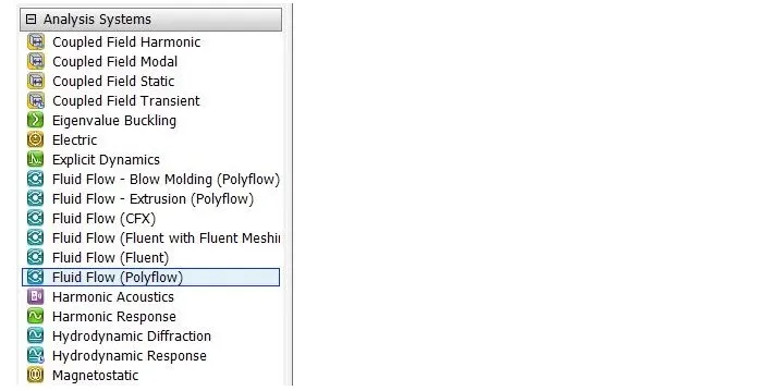
First, to make a simulation setup, select Fluid Flow(Fluent) from the left side window of the workbench.

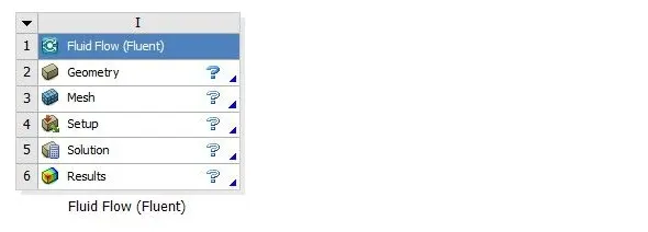
Next, select the first step which is to import geometry.

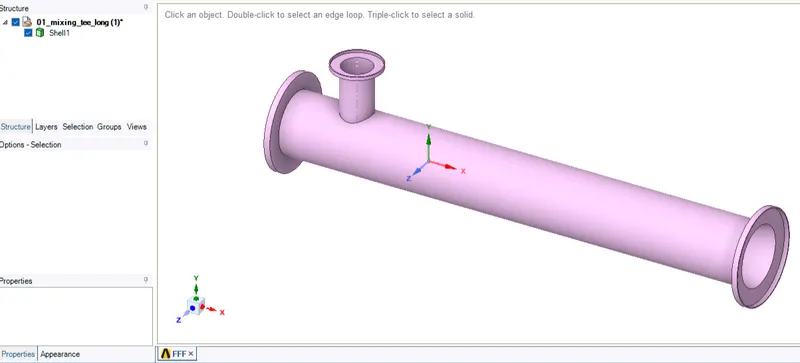
After opening the geometry, Select File ---> Open ---> and click the file that you wanted to open. Here, in this case, I have selected 'mixing_Tee_long.STEP'

Then click Prepare on the top menu bar to extract the volume that is needed for simulation.

After opening volume extract, click the edges from where the fluid flow is in contact during the simulation and remove the unwanted volume of the geometry by clicking the tick mark at the left bottom of the main window. Then, unbox the shell by clicking the tick mark in shell so that geometry which doesn't have the role to play during simulation is removed.

Then right click the shell and select supress for physics.

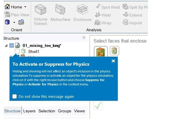
Once the geometry is complete, it shows tick mark in workbench geometry. After importing geometry, close the window and double click the mesh in the workbench. The window for mesh will open with imported geometry.

Mesh:

Now right click on the surfaces of the geometry and select Create named selection or press "N" as a shortcut key for naming the surface.

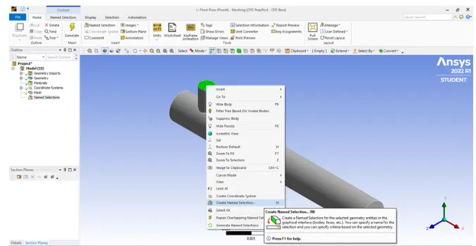
Now name selection box appears. Type name of the field in the name box.

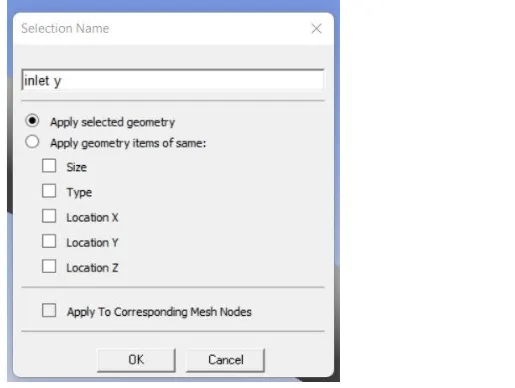
For inlet and outlet of the surface, give name as 'inlet (axis of the flow)' so that ansys can read the name and give the flow direction according to it during setup. example: 'inlet-x, inlet-y, outlet-x. Then select other surfaces and give name as 'walls'. Then close it before opening the next step 'SETUP'.

Then right click the 'mesh' and select update.

Setup:

Now double click the 'Setup' and open it. Tick the 'Double precision' check box and start the setup.

To change the units of the measurements, click units in the top left of the menu bar and select the units for the respective measurements.

For checking mesh, click 'mesh' --> 'Perform mesh check'.

Now, for selecting the type of model, select viscous in tool bar and select the model required and it's classification and its types.

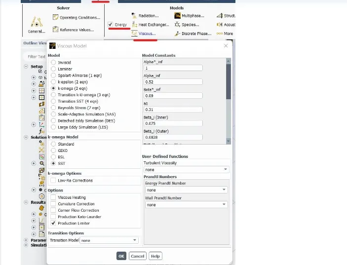
Then click the tick mark in 'Energy' check box since the temperature parameter is involved in simulation.

Now select 'boundary' in toolbar and select the surface where you have to setup the boundary conditions. The boundary conditions for temperature and velocity are inserted and apply ok.

Now click 'Defnitions' ---> New ---> Surface Report ---> Area-Weighted Average and

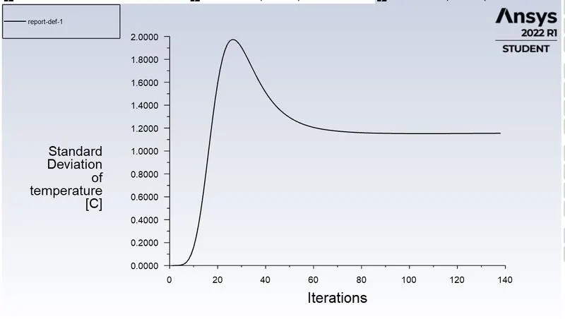
'Defnitions' ---> New ---> Surface Report ---> Standard Deviation.

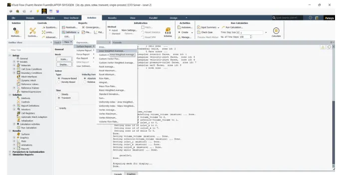
Then, click on initialize to initialze the data and click 'calculate' to perform iteration. Give the iteration number as 150 approx.

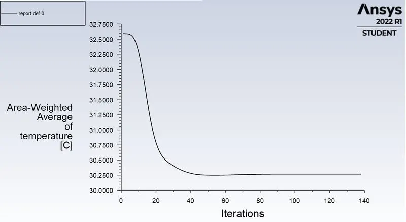
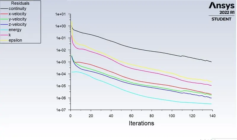
The 'Scaled residuals' and the 'Area-Weighted average of temperature' plots is displayed on the graphics window and in the console window, the iterations of the simulation is displayed.

Results:

After setup, close the window and click results to check and analyse the results of simulation.

The result window will open and the walls of the mesh will appear on screen after clicking the tick mark of walls.

Now click render icon and increase the value of transperancy to make the walls more transperant so that contour images of the flow can be viewed easily.

Now click 'Insert' icon in the menu bar ---> location ---> plane.

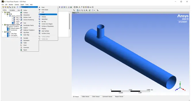
Now click in which plane the contour plot needs to be displayed in geometry section.

In the color section, change the mode to 'variable' and in the 'variable' portion, select the required variable such as temperature, pressure etc, in which the plot to be displayed. Then select 'Apply'.

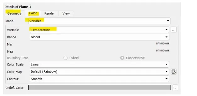
Then the required plot will be displayed on the screen in the entered plane of axis.

Solution:

To get the values of results of simulation, close the 'results' window and open the solution in the workbench window.

Now in the 'console' window of the solution, we can take the results such as

1. Cell count
2. Average outlet temperature
3. Number of iterations for convergence

The number of iteration for convergence is calculated by viewing the plotted graph from where after how many number of iterations, the slope of the line becomes zero is noted.

The above procedure is repeated for each case that is asked in question for both k-ε and k-ω model. So totally 8 simulations is carried on and the results are shown below.

	k-ε model				k-ω model
	Short mixing tee (3 m/s inlet velocity)		Long mixing tee (3 m/s inlet velocity)		Short mixing tee (3 m/s inlet velocity)		Long mixing tee (3 m/s inlet velocity)
	Momentum ratio=2	Momentum ratio=4	Momentum ratio=2	Momentum ratio=4	Momentum ratio=2	Momentum ratio=4	Momentum ratio=2	Momentum ratio=4
Cell Count	12692	12780	15727	15709	12780	12780	15727	15727
Avg.Temperature outlet	30.2668	27.50	30.2613	27.4830	30.262	27.574	30.306	27.494
No of iterations	50	40	60	50	60	50	80	40
Standard Deviation of temperature	1.1545	1.3502	1.2342	0.4698	1.555	1.422	0.9822	0.629

Velocity and temperature contour plots:

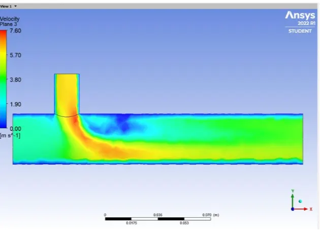
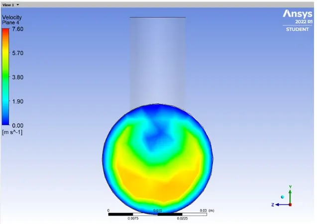
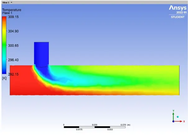
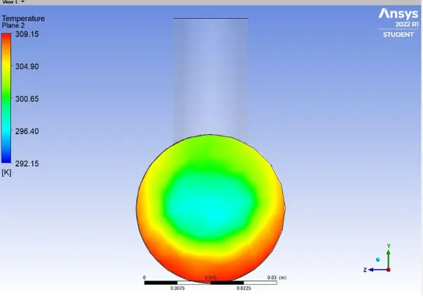
Model: k-ε model

Geometry model: Short mixing tee (3 m/s inlet velocity)

Momentum ratio: 2

Velocity contour plot along the pipe:

Velocity contour plot across the pipe:

Temperatue contour plot along the pipe:

Temperatue contour plot across the pipe:

Area-Weighted Average of temperature [C] line graph with respect to iterations:

Standard deviation of temperature line graph with respect to number of iterations:

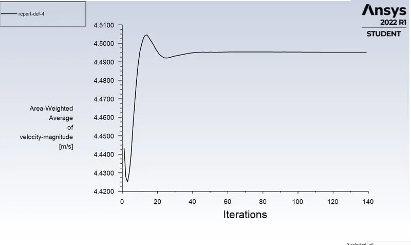
Area-Weighted Average of velocity-magnitude [m/s] line graph with respect to iterations:

Scaled residuals:

The same procedure is repeated for remaining 7 cases where we can get all the above mentioned results.

Mesh independent study:

The mesh independent study is performed for the below case.

Model: k-ε model

Geometry model: Short mixing tee (3 m/s inlet velocity)

Momentum ratio: 2

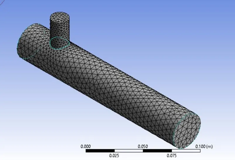
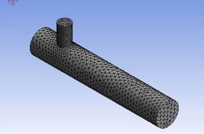
The mesh size of the above case is made finer with decreasing mesh size in each step. We have performed the case studies for 0.005,0.003,0.002,0.001 case studies for mesh independent study and results are tabulated in the table.

Mesh geometry with default element size:

Mesh geometry with element size of 0.005:

Mesh geometry with element size of 0.003:

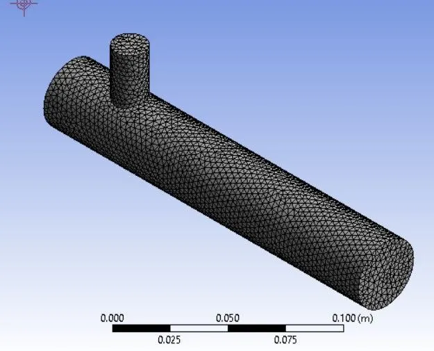
Mesh geometry with element size of 0.002:

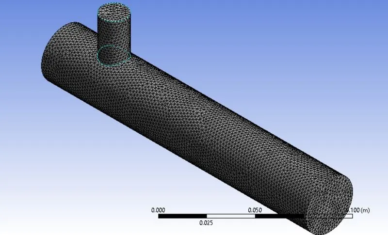
Results of mesh study:

k-ε model (01_mixing_tee_short.STEP)
Mesh Element size	Default size	0.005	0.003	0.002
Momentum ratio	2	2	2	2
Number of cells	12692	14249	39792	106544
Avg.Temperature outlet	30.266	30.247	30.273	30.297
Standard Deviation	1.1545	1.4168	1.6383	1.8407
No of iterations for converging	50	60	70	75

Error faced:

When reducing the element size further to 0.001, the following error is displayed.

Observation from the mesh study:

• From the above mesh refinement study, it is observed that the average outlet temperature of the case is found to be 30.2 degree Celcius and as the mesh gets finer, the average temperature at outlet temperature increases to negligible amount which states that it is diverging one.
• As the mesh size decreases, standard deviation increases beacuse as the number of cells increases, the temperature is calculated more accurately increasing deviation in calculated values from one cell to another cell.

CONCLUSION:

• To get better mixing at outlet, high velocity is preferred so momentum ratio of 4 has better mixing results at outlet.
• As the length of the mixing tee increases, the mixing time is more before it exits from the outlet. Thus the long mixing tee has better mixing characteristics.
• As the mesh size is coarser, the number of iterations required to converge to final result is less. But as the mesh size gets finer, the number of iterations for convergence increases since there are more number of cells to perform simulation.