Week 1- Mixing Tee

The objective of the following simulation is to set up the steady state turbulent cases for mixing tee with one inlet at hot temperature and another inlet at cold temperature. The aim is to find the effectiveness of mixing tee for two cases. First a short tee and the second one with a long tee. The results are depicted through the standard deviation of temperature, temperature contours, velocity contours and the area-weighted average of temperature. The simulation is backed with a grid sensitivity test. The parametric study is performed to explain the effect of length and momentum ratio on results.

K-Epsilon and K-Omega SST models are used for Reynolds stress modeling.

The cases are performed in steps of

1. Geometry and volume extraction
2. Mesh generation
3. Solver and physics setup with boundary conditions and Initial Conditions
4. Solution initialization and solution calculation
5. Post Processing with contours and reports

The cases are simulated below:

Case 1 -

1. Short Mixing Tee with a hot inlet velocity of 3m/s
2. Momentum ratio of 2.4
3. Th = 36 degC, Tc = 19degC

Step 1: Geometry Importing and Volume Extraction from Geometry

In this step Geometry of Short Tee is imported from Solidworks with extension .sldprt. After the opening of the geometry, We have to extract volume for the fluid simulation as this is a solid part but solid has no role in our simulation. Also, we suppress the solid body as it has no part in the present simulation.

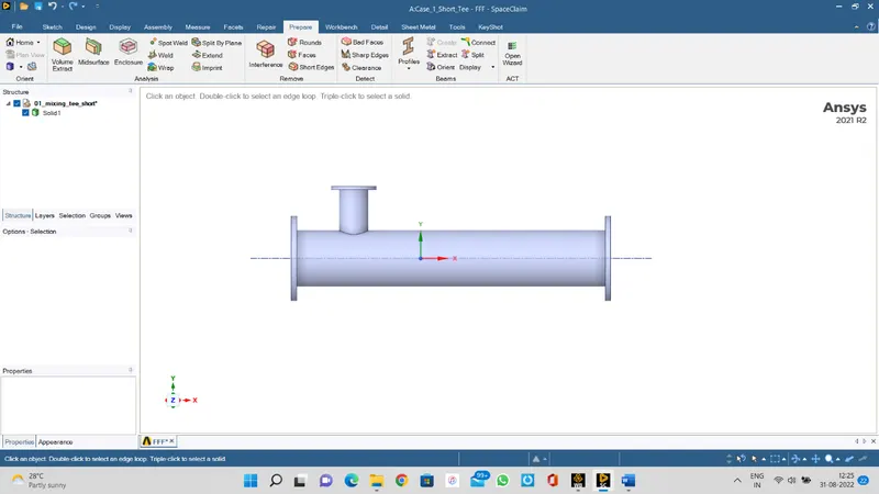
Volume Extraction

Volume is extracted under prepare option in spaceclaim with edge selection method.

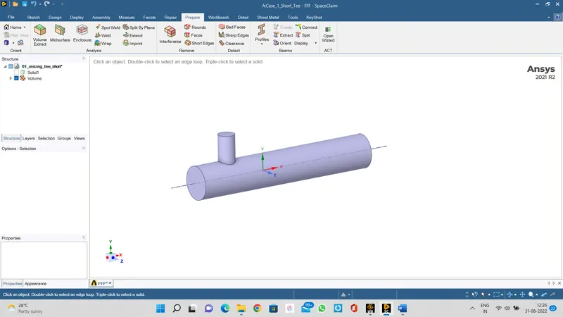
After this, our geometry is completed for the present simulation.

Step -2: Meshing

Now, open the mesh module in the workbench. 

In the mesh module, window, first we can create the named selection to name the boundaries for imposing boundary conditions and input conditions.

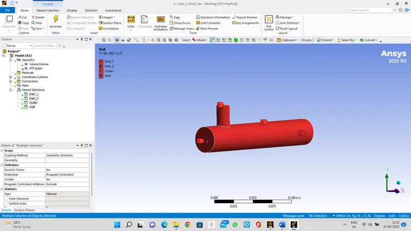
Now, firstly we generate the default mesh with the default element size, by right-clicking the mesh in the right pane and then click generate. The mesh quality and statistics are shown in the figure attached.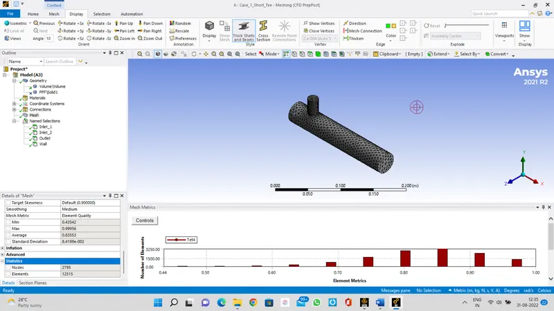

with this our mesh is completed, we can close the mesh module and go further for solver setup/

Step 3: Solver setup

Now, open the setup module in the workbench with simulation details of 3D, 2D, Precision details and processor details. IN the setup module first step is to select the materials and fluids used in the simulation. In our case we have taken air as the working fluid with properties inbuilt in fluent database.

Now we set up the physics of the problem, in this case, we select the steady state Pressure based solver, Checking the Energy on as we are dealing with temperatures. For viscous modeling, as we are there in turbulent conditions, we select K-Epsilon Realizable model for Reynolds stress modelling. After setting up the physics we are now in a position to setup boundary conditions based on given input conditions.

For hot inlet_1: Temperature = 36 degC, Velocity = 3m/s

For cold_inlet_2: Temperature = 19 degC, Velocity = 7.2 m/s

For outlet we select pressure oultet as BC

For walls we select wall boundary condition.

 

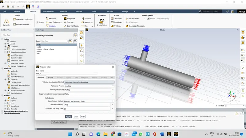
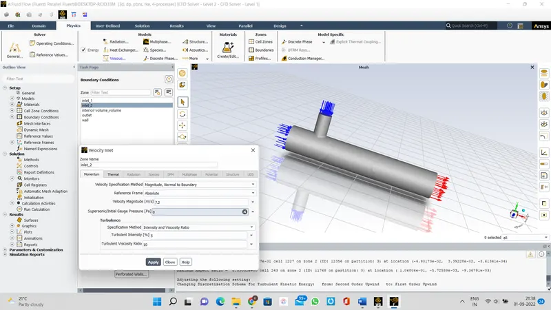
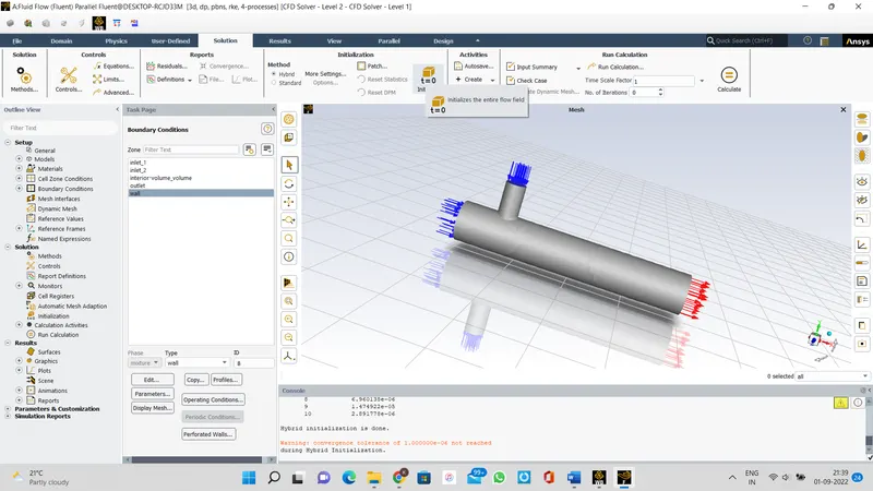
Now we initialize the solution.

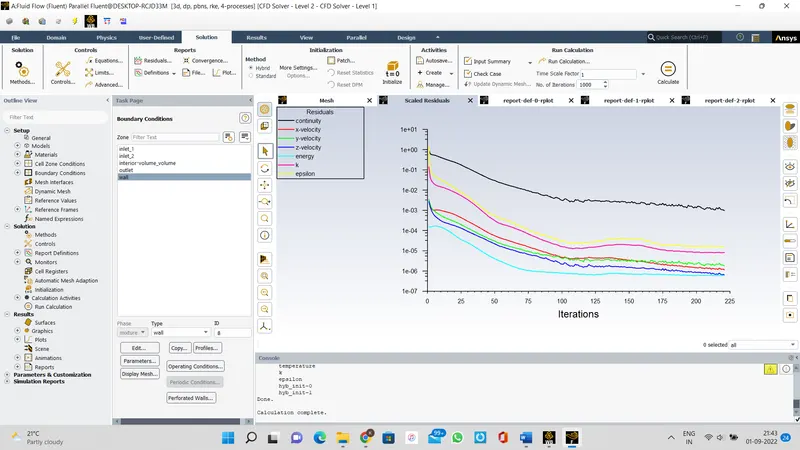
 Now we solve the solution for number of iterations and generate required reports.

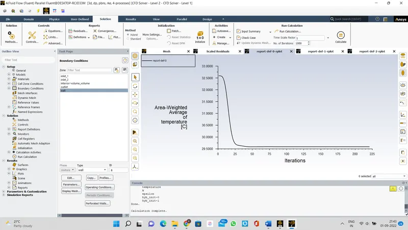
Report 1 Area weighted average of temperature at the oultet.

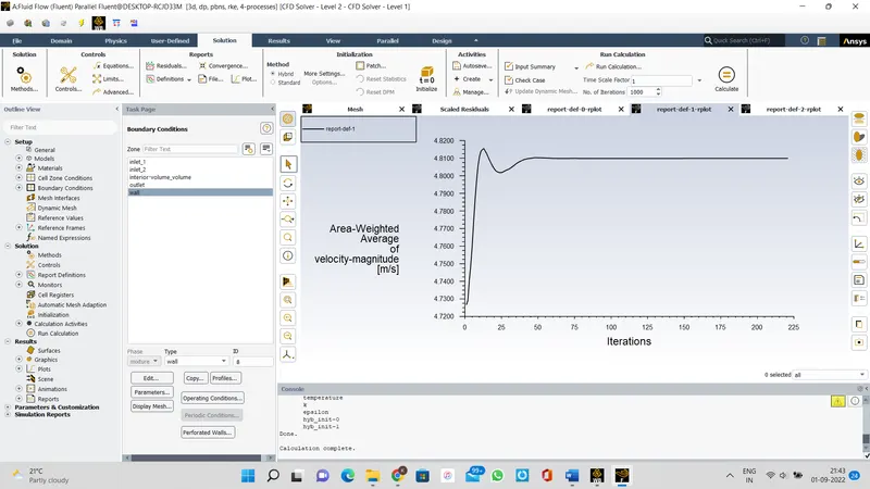
Report 2: Area weighted average of velocity at the outlet

Standard deviation of temperature at the outlet to check the effectiveness of mixing.

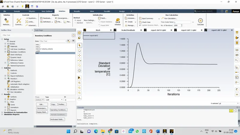
Note: The Solution is converged after 221 iterations for Case1 with 12515 cells of a mesh of default element size.

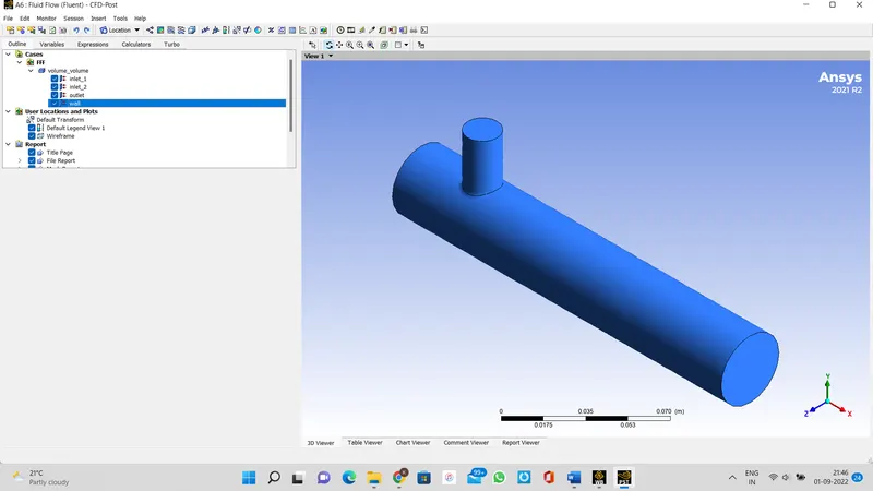
Now we can go to the CFD post to get the required plot and contours to depict the results.

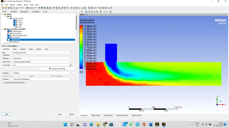
Temperature Contours:

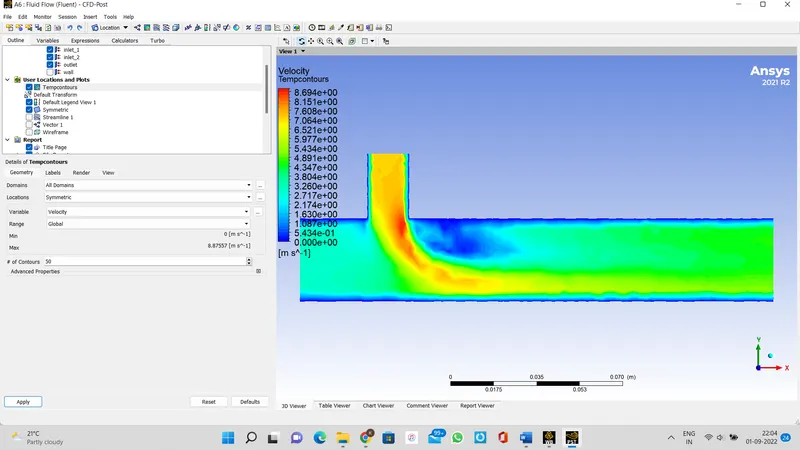
Velocity Contours:

 Now we will present the results for 

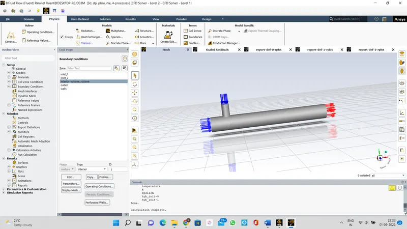
Case 2: Long Tee with similar BCs

Default Mesh size:

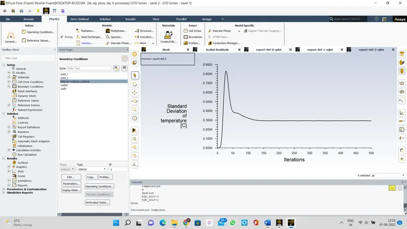
Standard Deviation for Temp

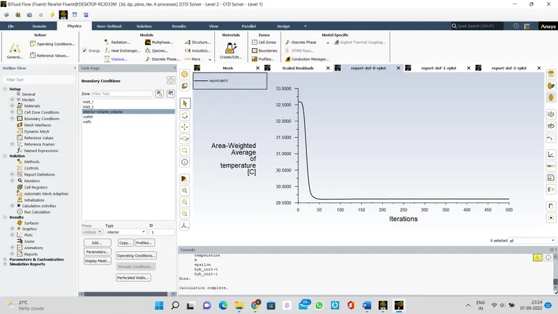
Area weighted Average temp for case 2:

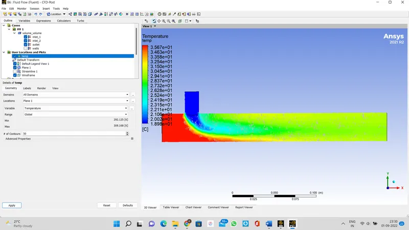
Temp Contours for Case2

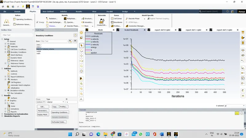
 For the default mesh size the convergence is not achieved for 500 iterations for Case2 as seen from residual plots that solution is oscillating.

 

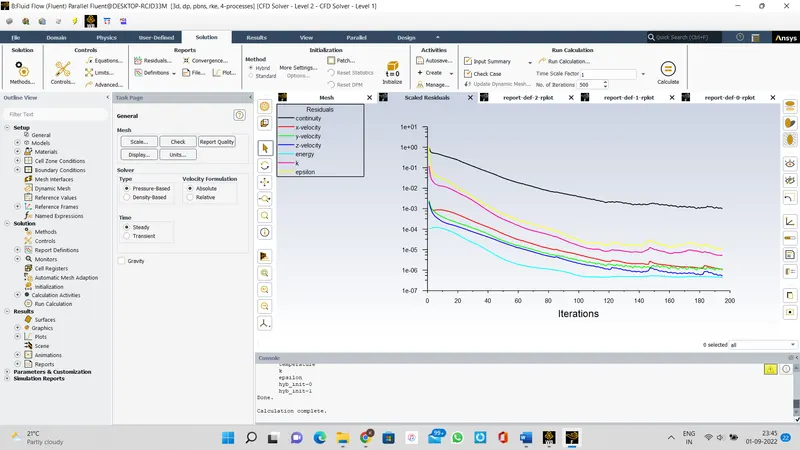
Therefore a fine mesh of element size 0.005 mm is taken to converge the solution and the solution converges at 191 iterations. The number of cells for fine case are 17565 as compared to default of 13575.

The converged solution details are:

Residuals:

Temp contours:

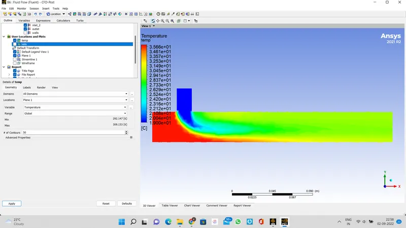
Conclusion:

It is seen from the above results that better mixing is obtained in the case of a long tee case. As the standard deviation for a long tee is less and also it can be seen from the contours that uniform temp is obtained at the outlet.