Week 1- Mixing Tee

                                                              Mixing Tee

AIM: To set up steady-state simulations to compare the mixing effectiveness when the hot inlet temperature is 36⁰C & the Cold inlet is at 19⁰C creating two versions of the mixing tee.

Objective:

• To clean the geometry and mesh it in pre-processing.
• To solve the model with best solver in Ansys solver.
• To generate contour and line plots and analyse it in postprocessor.

1. Case 1 
   • Short mixing tee with a hot inlet velocity of 3m/s.
   • Momentum ratio of 2, 4. 
2. Case 2 
   • Long mixing tee with a hot inlet velocity of 3m/s.
   • Momentum ratio of 2, 4.

• Momentum ratio = velocity at cold inlet / velocity at hot inlet
• In a table, compare the following values from the 2 cases. 

1. Cell count
2. Average outlet temperature
3. Number of iterations for convergence

• Expected results:

1. Velocity and temperature contour plots on the cut planes along and across the pipe.
2. Velocity and temperature line plots along and across the length of the pipe.
3. Perform Mesh independent study for any one case.
4. Discuss the effect of length and momentum ratio on results. 

INTRODUCTION:

The function of mixing Tee is to provide proper mixing of quantities to get the desired result at the outlet.

 

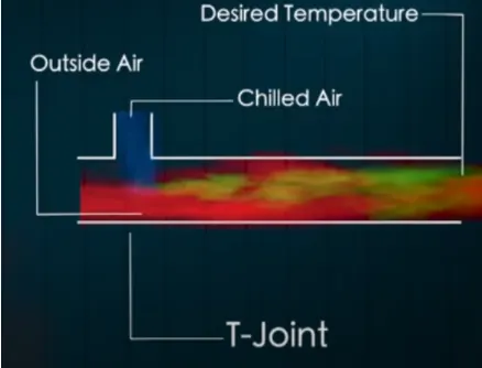
By controlling the velocity of chilled air we can get the desired temperature in the room.

ANSYS WORKFLOW:

 

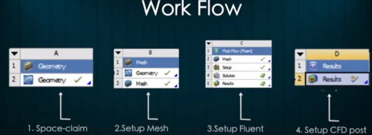
GEOMETRY: Construct a two or three dimensional representation of the object to be modelled and tested using the work plane coordinate system within ANSYS.

MESH: At this point ANSYS understands the makeup of the part. Now define how the modelled system should be broken down into finite pieces.

SETUP: The case setup will be done using ansys fluent.

SOLUTION: Ansys fluent where run time result visualization is done.

RESULTS: Post processing of results will be done here using CFD-post.

Procedure:

1.Open new project, by clicking on Fluid flow (Fluent) in Ansys workbench.

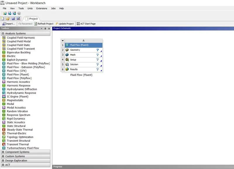
                                                                         Fig. Ansys Workbench - New Project

2. Now click on geometry to import mixing tee model. It will redirect to Spaceclaim, Ansys’s geometry model manipulator.

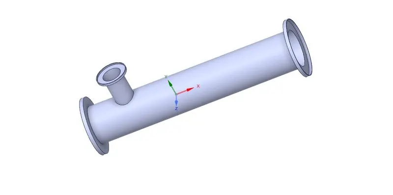
                                                                  Fig. Imported Mixing Tee Model

3. We are to analyse the mixing of two fluid, so there is role of parts other than two pipes. To supress that we need to extract volume of tee. Go to prepare menu and click on volume extract. Switch to edge selection and select three outer edges and click on green check button.

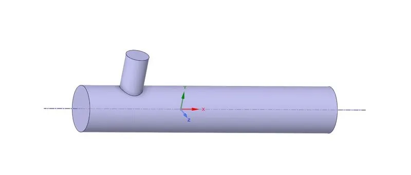
                                                                     Fig. Extracted Volume

4. Hide solid by unchecking it from structure menu to see volume, which we have extracted. Supress solid by clicking on option supress for physics.

5. Exit from Spaceclaim and click on mesh to open mesh menu.

6. Select outer face and press right click of mouse, it will open a menu. Click on option create named selection and write suitable name for face. Repeat for other faces.

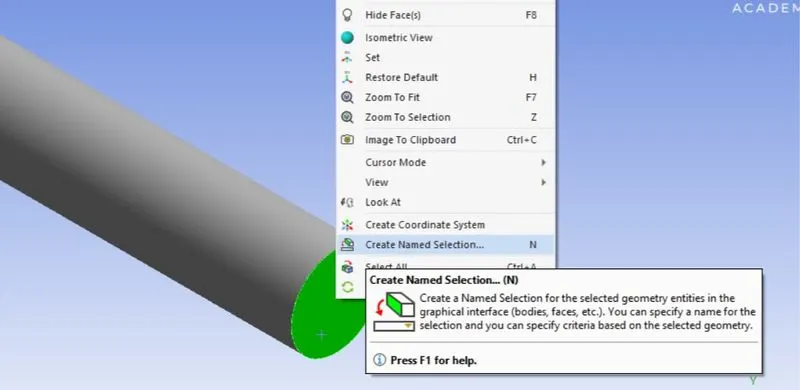
                                                                   Fig. Creating Faces Name

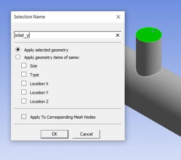
                                      Fig. Selection Name Menu

7. Now click on mesh option and choose generate mesh. It will generate mesh according to some predefined criteria. Element size can be selected but it is going to affect simulation time. Section plane can be created to see inner portion of geometry.

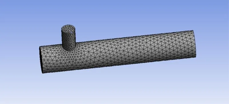
                                                                     Fig. Generated Mesh

8. Select the option element quality to see, how many elements are defying quality. Quality is measured on the scale of 0 to 1. In our graph most of the element are near to 1 so we can say it is good quality.

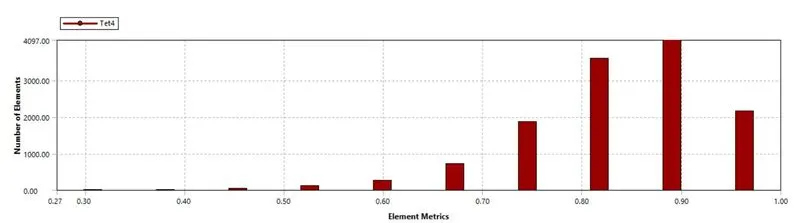
                                                          Fig. Number of Elements vs Element Metrics

9. Exit mesh and open setup. First, Check mesh, it is throwing no error then only we can proceed further. We are going to do pressure based steady state simulation, so choose these options on task page.

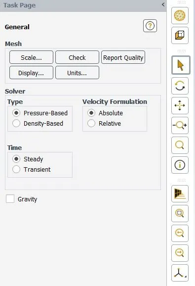
                              Fig. Task Page

10. Go to physics menu and select viscous model. It will open a menu, choose realizable k-epsilon model and close it.

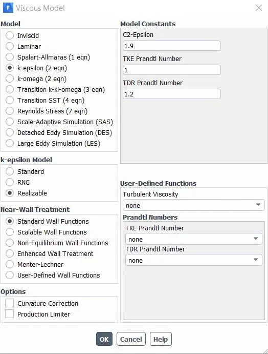
                       Fig. Viscous Model Parameters

11. Click on material and choose air as working fluid. Check working fluid by clicking on cell zone conditions option, if it is air then proceed.

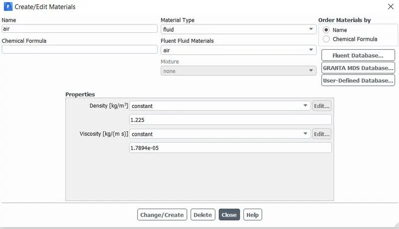
                                                                      Fig. Assigning Material

12. Now go to boundaries option to set boundary conditions. Select inlet_x and click on option edit. It will open a menu, where all the parameter can be set whether it is thermal, radiation, momentum etc. Put the value of velocity as 3m/s and go to thermal parameter to set temperature as 36C, for hot fluid.

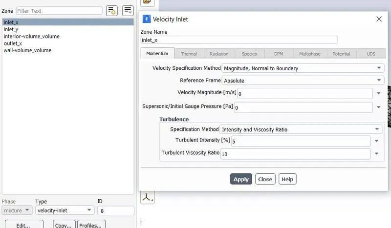
                                                                 Fig. Applying Boundary Conditions

13. Repeat the same procedure for cold fluid coming, velocity –6 m/s, temperature – 19C.

14. We want to generate temperature report of outlet and we want standard deviation of temperature also. Go to solutions tab and select definition and select area weighted average. In the opened menu select temperature as field variable. Similarly select standard deviation in definitions menu.

15. Now click on initialization to calculate approximate values of velocity and pressure.

16. Change the number of iterations to 250 and click on calculate. If solution is not converged, then iterations can be increased.

17. Exit setup and double click on result to open CFD post. Check boxes to see walls and other parts. Click on walls and go to render set transparency of 0.4 to inside of wall. Colour can also be changed to white for clear visibility.

18. Now insert a XY plane in wall by clicking on plane in location option of insert.

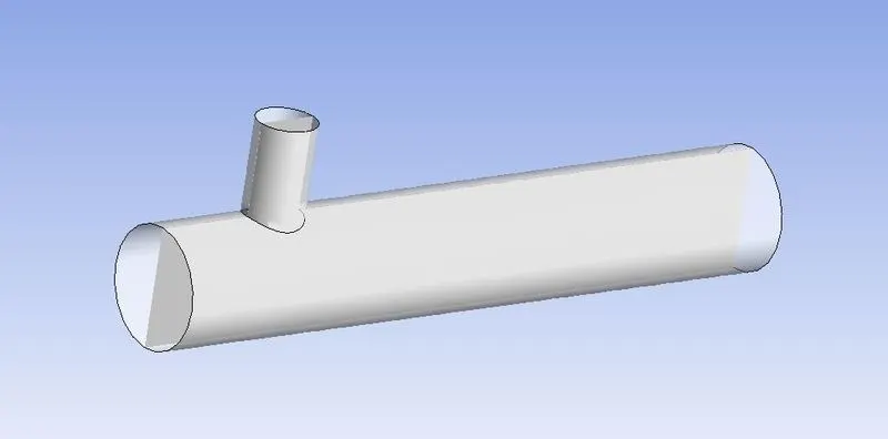
                                                         Fig. Transparent Mixing Tee with XY plane

19. Go to colour of plane and change it by variable choose option temperature. Similarly, velocity contours can be created by just changing variable as velocity.

20. Right click on plane which we created and select streamline. Go to appearance and select temperature to see plot line on plane. Similar procedure can be repeated for velocity plot line.

 Results –

Case 1 – In this short mixing tee is used, which was mixing two fluid with temperature 6C and 19C. Velocity of hot fluid was 3m/s and cold fluid was 6m/s. we used two different turbulent solvers for it first was realized k-epsilon and second was k-omega SST.

In this case k-epsilon is giving better results because solution was converged after few iterations, whereas after using k-omega model solution was not converged. K-omega is preferred in studying fluid behaviour near wall, but here it is not the case. So, k-epsilon model is recommended to study of fluid far from wall i.e. flow region, in further cases.

Plot and contours from k-epsilon model

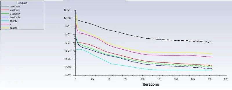
                                                                       Fig. Residuals

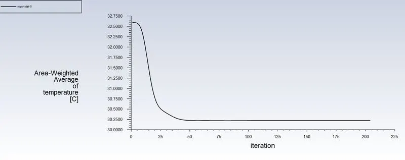
                                                                        Fig. Average Temperature vs Iterations

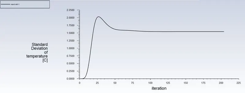
                                                                    Fig. Standard Deviation of  Temperature vs Iteration

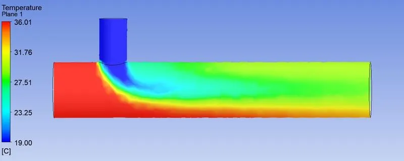
                                                                      Fig. Temeprature Contour

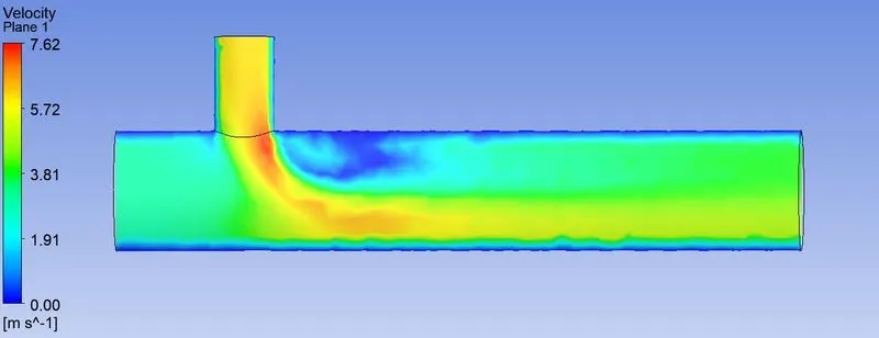
                                                                         Fig. Velocity Contour

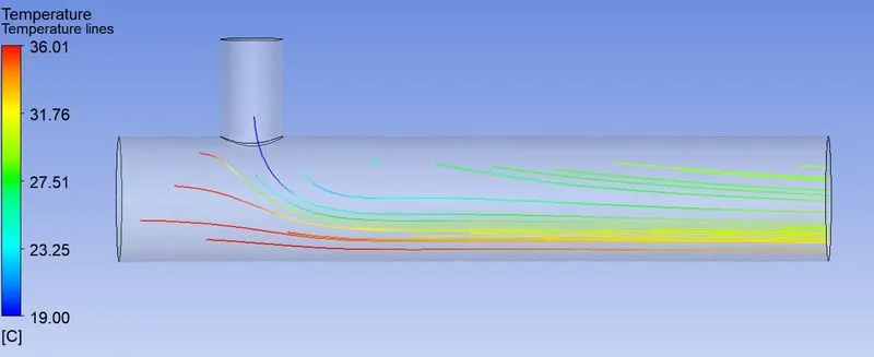
                                                                       Fig. Temperature Streamline

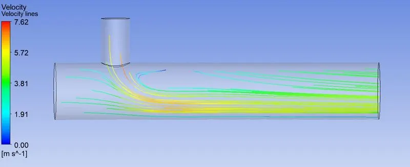
                                                                       Fig. Velocity Streamline

 Plot and contours from k-omega model

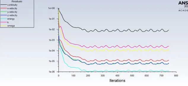
                                                             Fig. Residuals

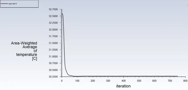
                                                                              Fig. Average Temperature vs Iterations

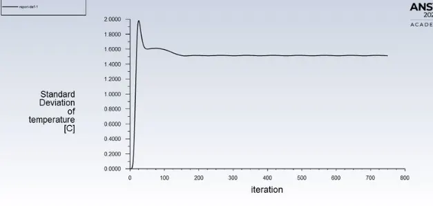
                              Fig. Standard Deviation of  Temperature vs Iteration

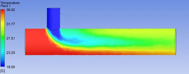
                                                                      Fig. Temeprature Contour

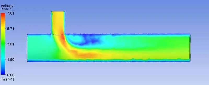
                                                                         Fig. Velocity Contour

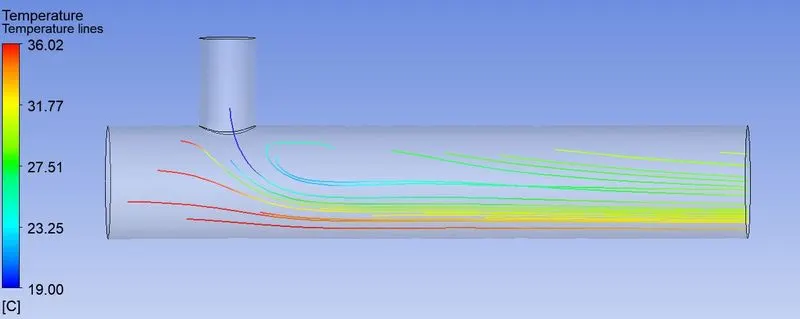
                                                                       Fig. Temperature Streamline

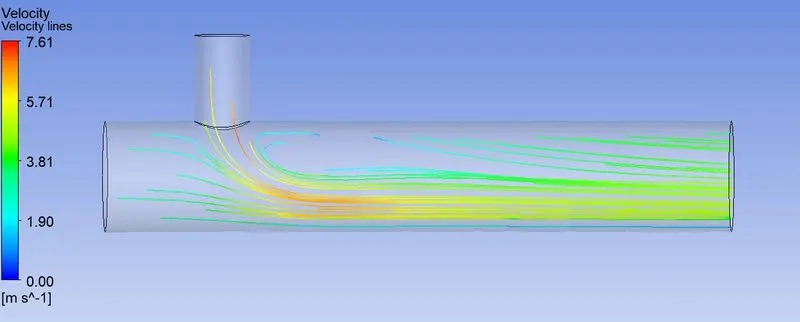
                                                                       Fig. Velocity Streamline

Case 2 - In this case long mixing tee is used, which was mixing two fluid with temperature 6C and 19C. Velocity of hot fluid was 3m/s and cold fluid was 12m/s.

We used realized k-epsilon model and solution was converged after 156 iterations.

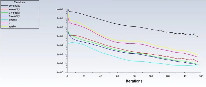
                                                                     Fig:Residuals

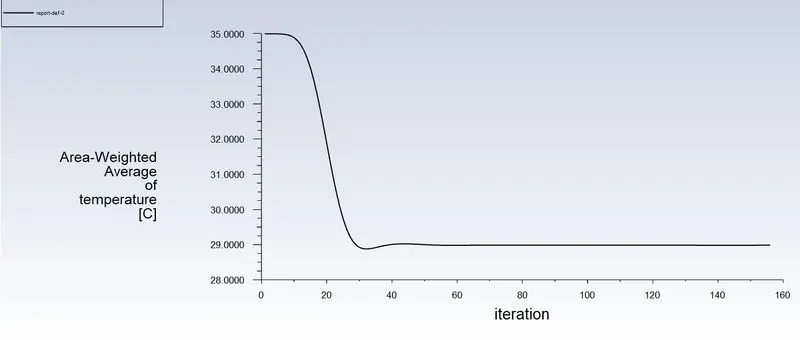
                                                            Fig. Average Temperature vs Iterations

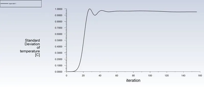
                                                   Fig. Standard Deviation of  Temperature vs Iteration

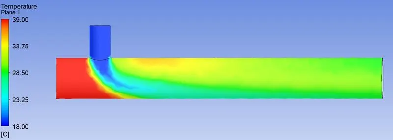
                                                                 Fig. Temeprature Contour

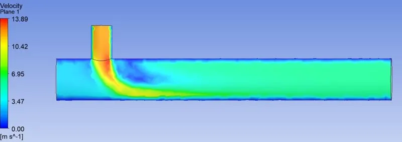
                                                                     Fig. Velocity Contour

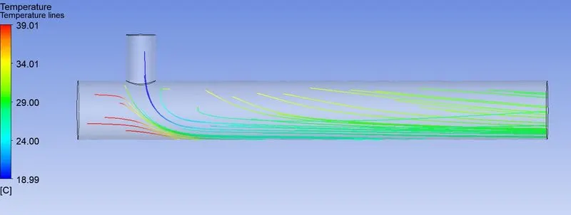
                                                                 Fig. Temperature Streamline

                                                              Fig. Velocity Streamline

Comparison table –

Parameters	Cell Count	Average outlet temperature	Number of iterations to converge
Case 1	12812	30.20C	199
Case 2	15588	29C	157

Mesh Independent Study –

Mesh independent test allows mesh refinement without affecting results. After some tests we can be ensured by solution that mesh refinement won’t affect the result. The following graphs are showing the results after mesh refinement on short mixing tee, earlier element size is used as 0.0195 and now it got 0.001.

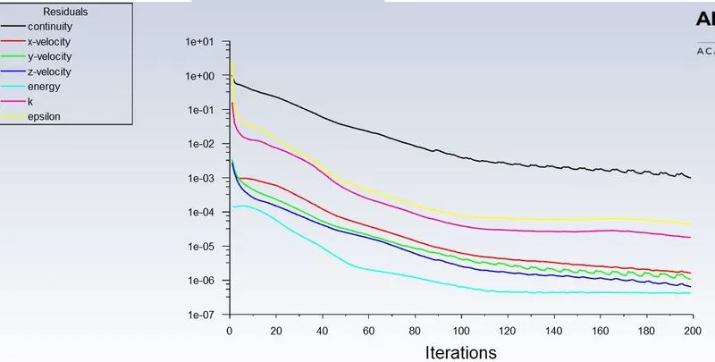
                                                                        Fig. Residuals

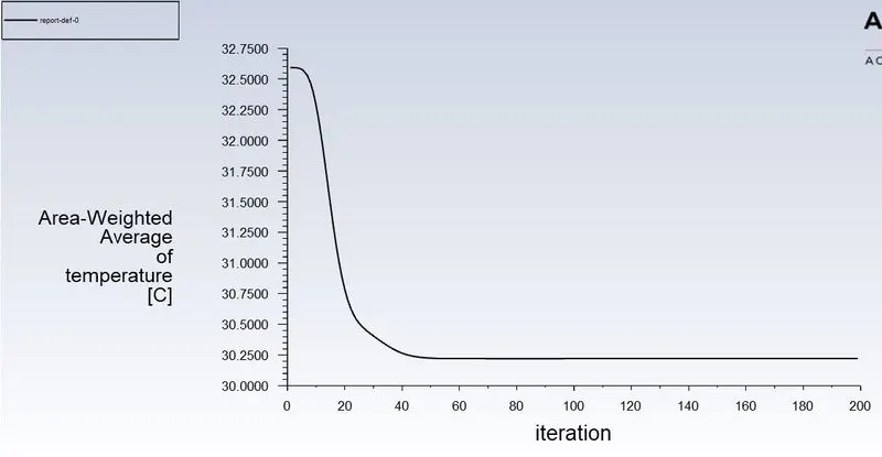
                                                               Fig. Average Temperature vs Iterations

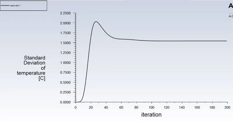
                                                           Fig. Standard Deviation of  Temperature vs Iteration

CONCLUSION:

• k-epsilon models predict flow virtually far from the boundaries (wall), and the k-omega model predicts near the wall. As in this case we need a flow simulation turbulent model far from the wall, therefore, the k-epsilon method is used.
• Solving the first simulation on the fluid domain using coarse mesh gives an initial overview of the analysis which converges results fast. As element number increases the convergence time also increases. Therefore, after obtaining the rough results using coarse mesh simulation successfully we can improve mesh quality and get to final accurate results doing this saves a lot of time which is also extremely helpful for mesh independence test.
• To get better mixing at outlet high velocity of flow is very effective. Therefore, a higher momentum ratio gives better mixing of hot and cold fluid stream at the outlet.
• As the Length of the mixing tee increases because diffusion flow always gives slightly better mixing of two-fluid.
• Finally, in the above cases, it is very important to use a short mixing tee with a momentum ratio of 4 to get precise results but one has to consider the diffusion of flow along the length of the mixing tee, a long mixing tee with momentum will be the greater option.