Week 1- Mixing Tee
Project: Steady Simulation of Mixing with Turbulence Modelling
Objectives:
- To perform Mesh independent study for the case
- Discuss the effects of the momentum ratio and length of the pipe
- To compare the `k-epsilon and k-omega` Turbulence Model
- Velocity and temperature line plots along and across the length of the pipe
Aim: To Predict the Dynamics response of the Temperature when two different temperature identical fluids mixing together.
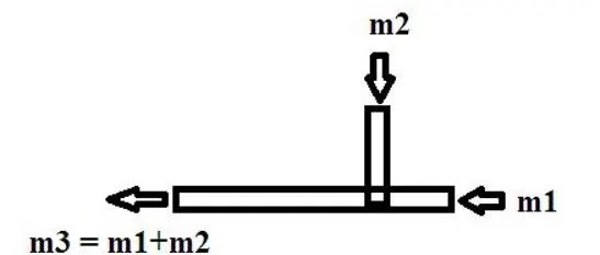
The application of the Mixing tee is found in various applications like Heat, Ventilation, and Air condition. The mixing of the two identical fluids is discussed here. Where the Real fluids mixing temperatures given by
`T_(mixture)=(c_(p_1)*m_(hot)*T_(hot)+c_(p_2)*m_(cold)*T_(cold))/(c_(p_1)*m_(hot)+c_(p_2)*m_(cold))`
Where the Identical the specific Heat capacity of two fluids are equal.`c_(p_1)=c_(p_2)`
`T_(mixture)=(m_(hot)*T_(hot)+m_(cold)*T_(cold))/(m_(hot)+m_(cold))`
On solving the above equation, Analytical
The flow inputs are hot inlet `36^oC` and cold inlet `19^0C`
Momentum Ratio is 2, 4 and mass flow rate`dot m_(hot)=rhoA_(hot)V_(hot)`
A mass flow rate of the cold fluid is `dot m_(cold)=rho*A_(cold)*V_(cold)`
Calculation for the Momentum Ratio=`V_(cold)/V_(hot)=2`
`m_(hot)=rho*A_(hot)*V_(hot)=1.225*901.3151*3*10^(-6) = 0.003312`
`m_(cold)=rho*A_(cold)*V_(cold)=1.225*225.9824555*6*10^(-6) = 0.001660969`
`T_(mixture)=30.32209^oC`
Calculation for the Momentum Ratio 4
`m_(hot)=rho*A_(hot)*V_(hot)=1.225*901.3151*3*10^(-6) = 0.003312`
`m_(cold)=rho*A_(cold)*V_(cold)=1.225*225.9824555*12*10^(-6) = 0.003321942`
`T_(mixture)=27.4872^0C`
Numerical Solving the Mixing tee with the coarse mesh include the following steps
- Volume Extraction
- Mesh and Check the Element Quality
- Solver and Computation
- Post Processing the Results
Volume Extraction :
It helps to extract the fluid volume. Here we do only to the Fluid flow study so the Solid part of the part is emitted. It is easily done by the Spaceclaim volume Extraction option
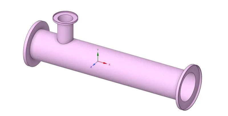
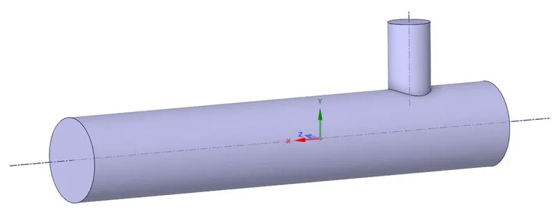
Mesh and Element Quality
Meshing is the process of dividing the domain into small fractions. Element Quality is checking the small fraction of the domain. It is kept as the Default as in the Fluent.
| Element Size | `1.0219e-2 m` |
| Nodes | 2783 |
| Elements | 12441 |
Element Quality is checked using the mesh Metrics Option

- It shows the Element quality is above 30% and More number of element quality is more 80%.
- This Mesh is good to run the simulation.
Solver and Computation:
- Close the Meshing application Open the Fluent for the further steps
- Check the model for the tick, if not update the mesh in the Workbench. Open the Fluent.
- Check the Mesh and Assign the required units.
- Setup the solver as Pressure Based, Velocity Absolute, and steady-state simulation.
- As we need to solve for the Temperature we are using the Energy Equation
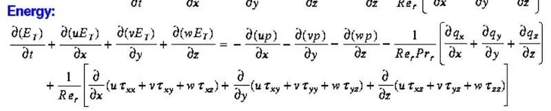
- We can solve the Navier strokes Equation directly but the Reynolds number should be in the order of `10^3` but the practical case Reynolds number at that, we need the more finer mesh and it takes lot of the computational time, because of this it is pretty much impossible to do for the real engineering problem like this. So we are using the Turbulence Model to achieve the similar results.
- Hereby, I have tested for the `k-omega and k-epsilon` Model.
- Next step is assigning the Boundary Condition to the model.
Inlet Cold Velocity 6 m/s or 12 m/s Inlet Hot Velocity 3 m/s Inlet Cold Temperature `19^oC` Inlet Hot Temperature `36^oC` Outlet Pressure 1 atm - Here I have done Hybrid Initialization to apply the Initial Condition.
- By defining the Area Weighted average and standard deviation.
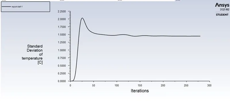
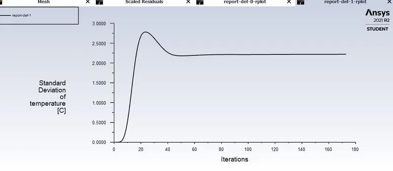
- By having a low standard deviation, we have an accurate solution.
- After the Computation, post-processing is done.
Post Processing:
`k-epsilon` (Realizable)
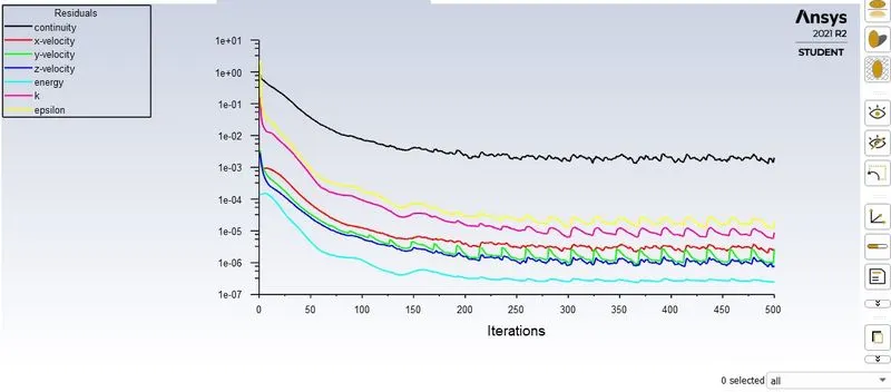
The figure above Residuals for the Governing Equation and Turbulence Equation.
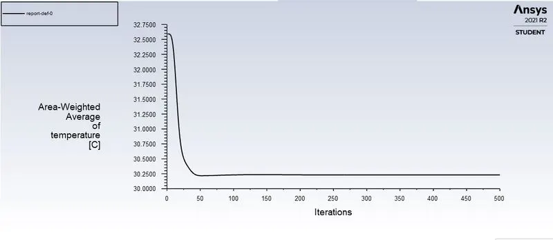
The figure above Area Weighted Average of the Temperature
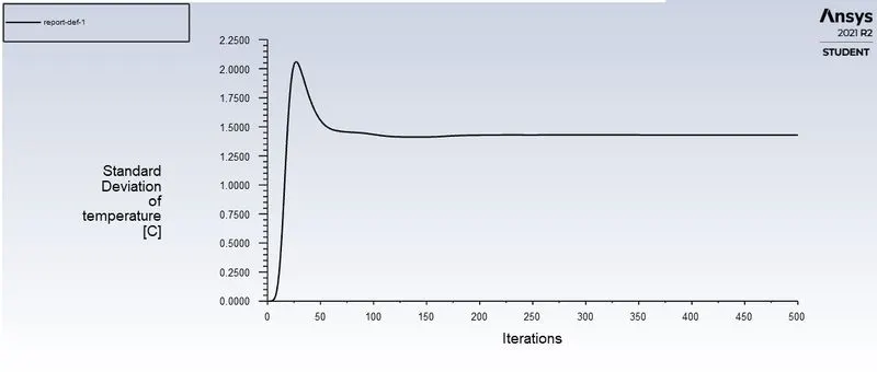
The above figure gives the Standard Deviation of the Temperature
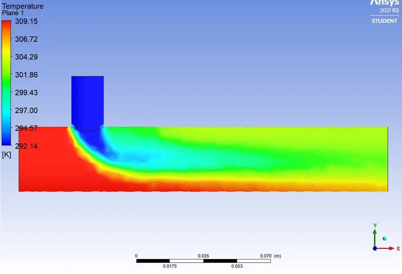
The above figure gives the Temperature plot.
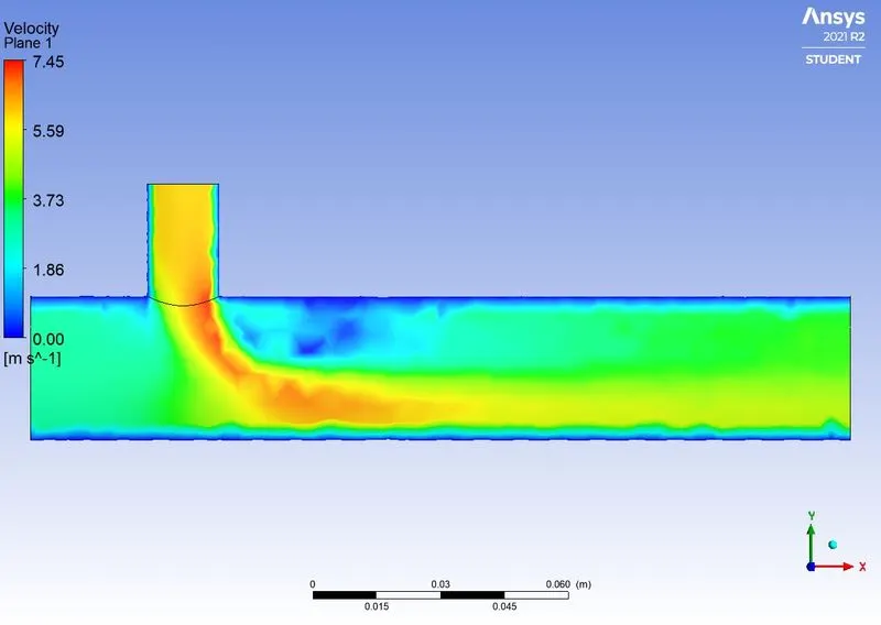
The above figure gives the Velocity plot.
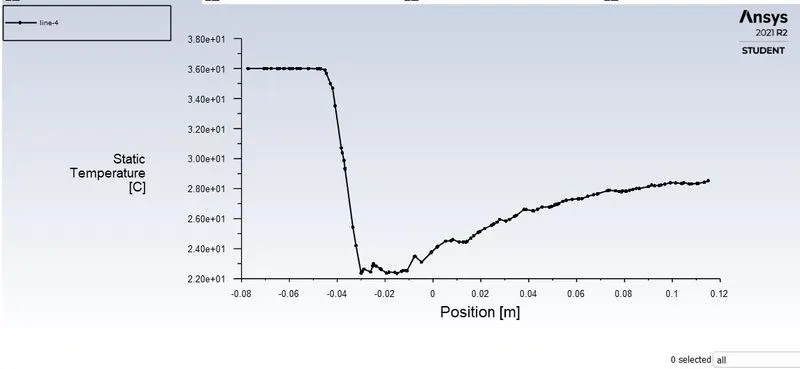
The above figure gives the Temperature over the length of the pipe.
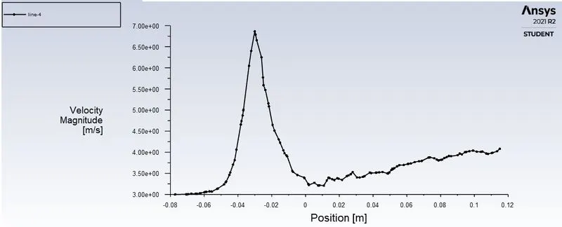
The above figure gives the velocity plot over the pipe.
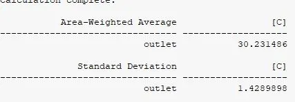
The Area Weighted Average temperature of the outlet is `30.231486^0C` for the `k-epsilon` Realisable.
`k-omega`
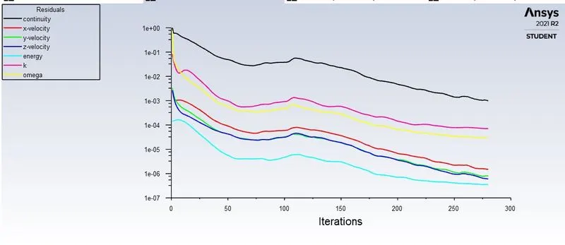
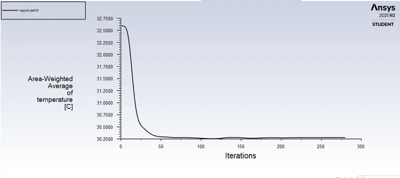
it converged at 280 Iteration
Residuals
Area Weighted Average Temperature
Standard Deviation
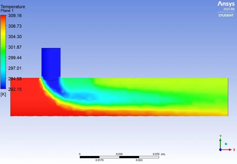
Temperature Plot
Velocity Plot
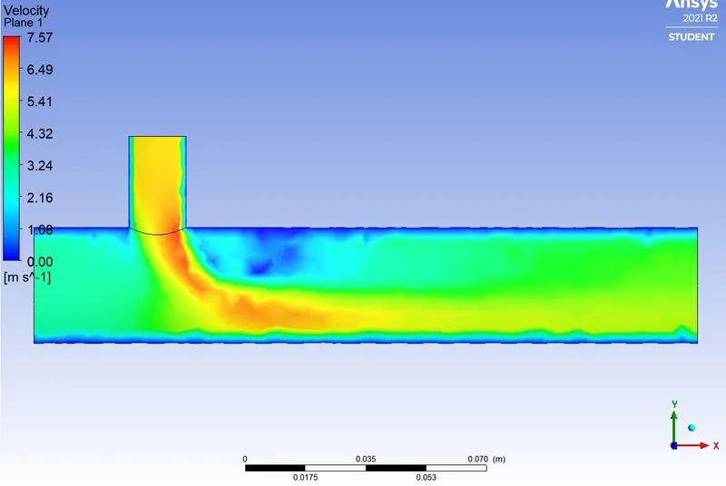
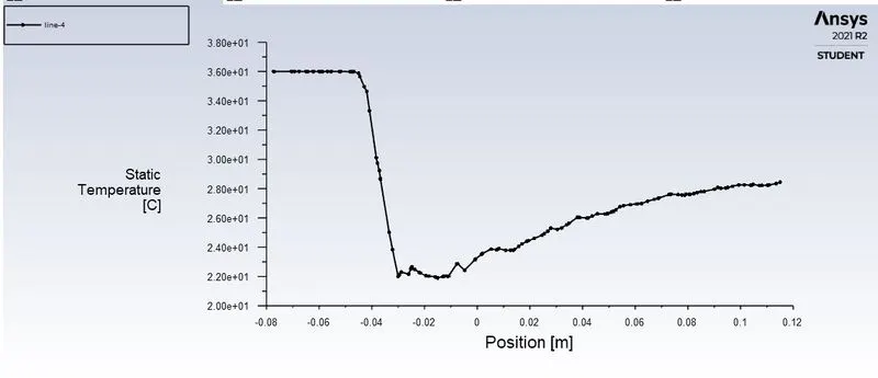
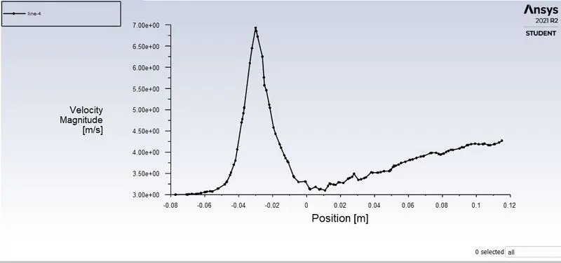
The following Figure gives the Temperature and Velocity plot over the pipe
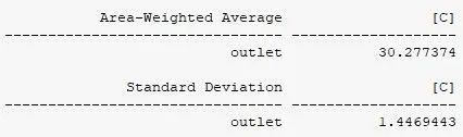
The Area Weighted average temperature of the outlet is given by
From the above Observation
- `k-epsilon and k-omega` model, from the model the k-omega SST Model predicts better turbulence model compare with the k-epsilon.
- K-omegaSST Model predicts the solution in less computational time than the k-epsilon.
- Hence we going with the K-omega SST Model
CASE-1(MOMENTUM RATIO 2) FOR THE MIXING SHORT TEE
Pre-Processing has done as same as the Coarse Mesh, Finer mesh is generated using the small Element Size.
| Element Size | `1.25e^-3m` |
| Node | 64281 |
| Elements | 329296 |
Results :
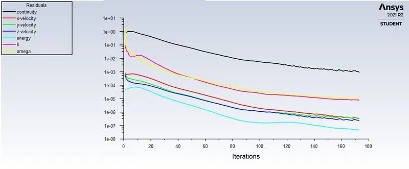
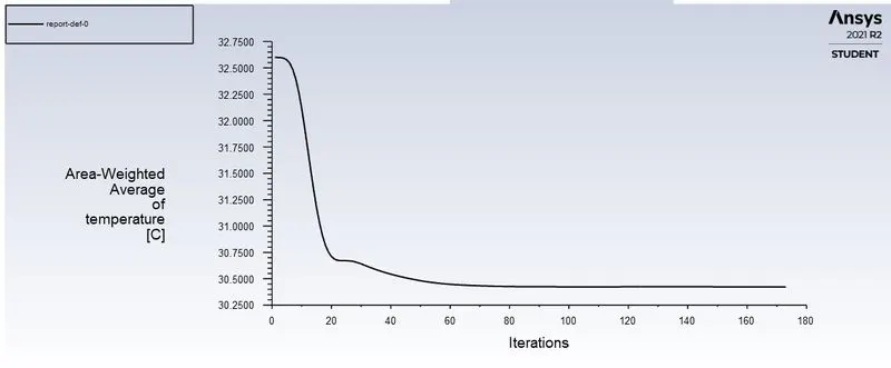
The solution is converged at the 173 Iteration.
Residual of the Transport and Governing Equation is given by
Area Weighted Average of Outlet Temperature is given by
Standard Deviation of the Temperature of outlet is given by
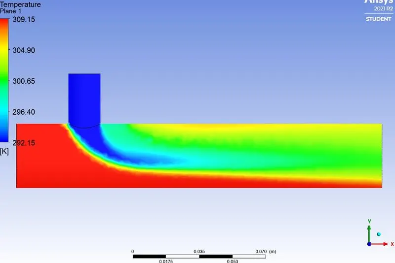
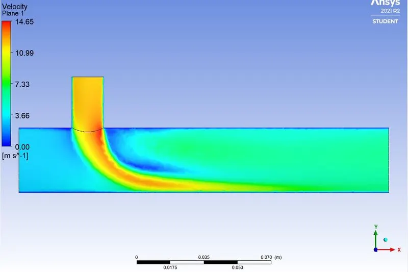
Temperature Plot of the Pipe
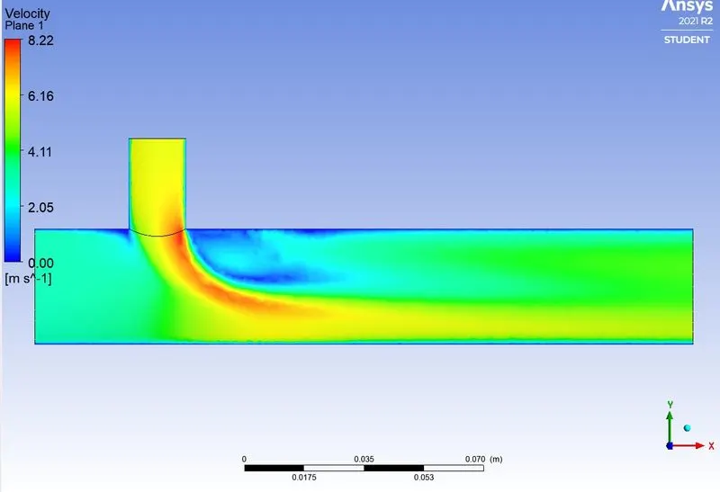
Velocity plot is given by
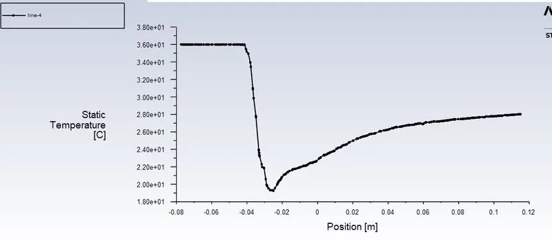
Temperature vs Length plot
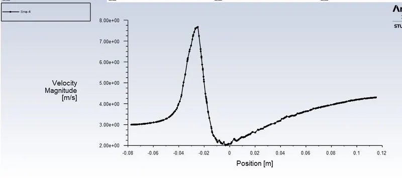
Velocity vs Length Plot
Numerical Results of the Outlet Temperature
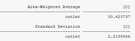
- Compare with the Analytical Temperature calculated from the formula is `T_(mixture)=30.32209^oC`.
CASE-2 Momentum Ratio 4 for Short Mixing Tee
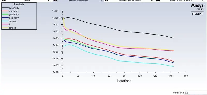
The solution is converged at 143 iterations.
Residual for the governing and transport Equation
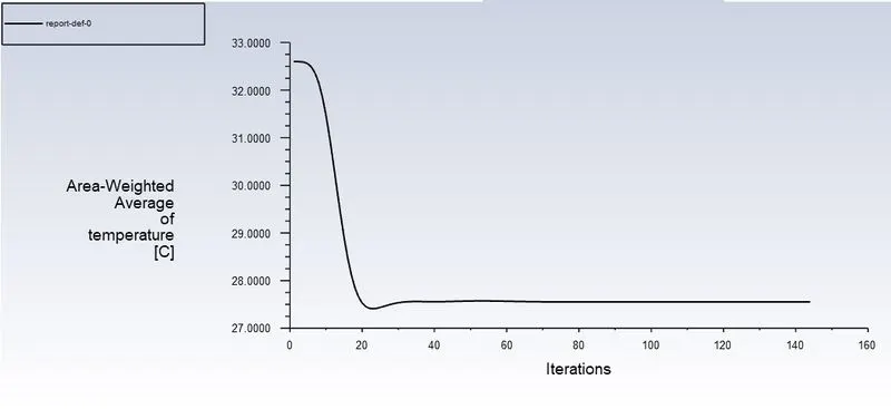
Area Weighted Average Temperature is given by
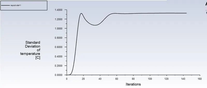
Standard Deviation of the Temperature of outlet is given by
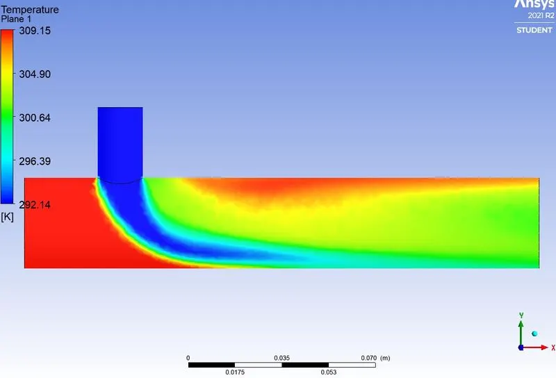
Temperature Plot of the Pipe
Velocity plot is given by
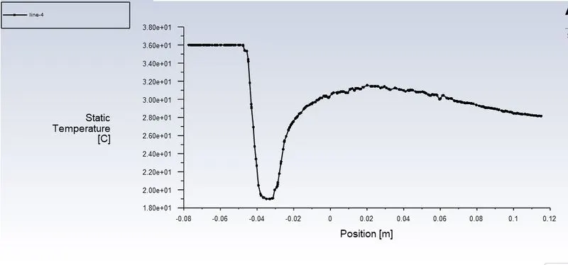
Temperature vs Length plot
Velocity vs Length Plot
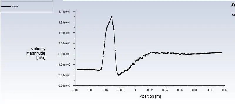
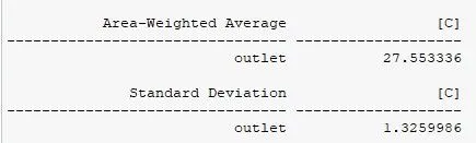
- Compare with the Analytical Temperature calculated from the formula is `T_(mixture)=27.4872^0C`
Case-3 (Momentum Ratio 2) For Long Mixed Tee
- Preprocessing models are prepared, based on the following information
| Element Size | `1.3e^-3` |
| Nodes | 79461 |
| Elements | 406876 |
- The solution is converged at 143 Iterations,
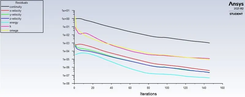
The Residual for the governing Equation and Transport Equation is given by
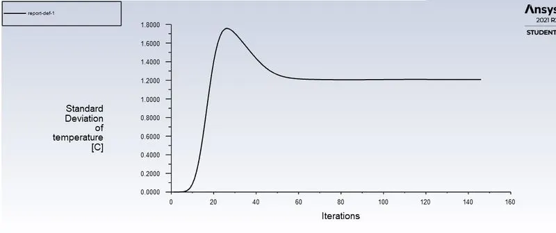
Standard Deviation of the Temperature of outlet is given by
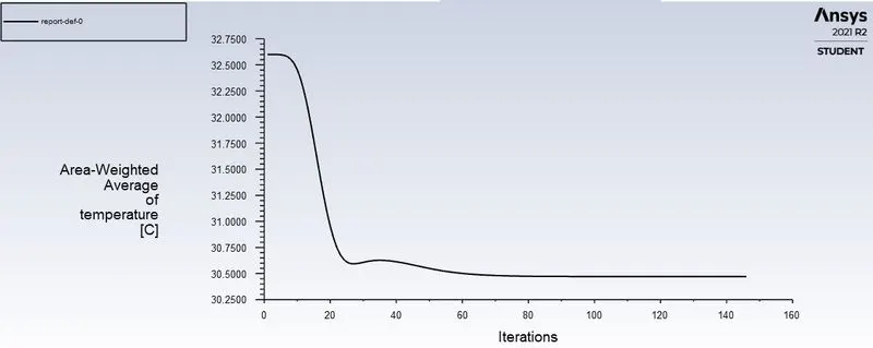
Area Weighted Average of Temperature Outlet
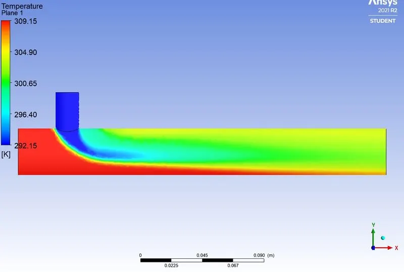
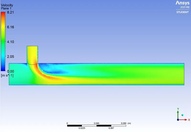
Temperature plot is given by
Velocity Plot is given by
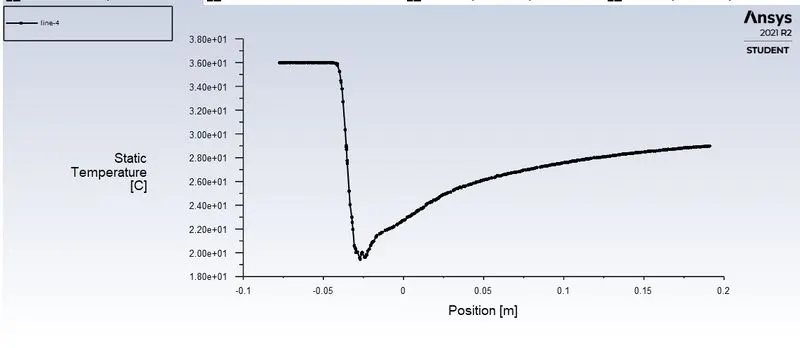
Temperature vs Length plot
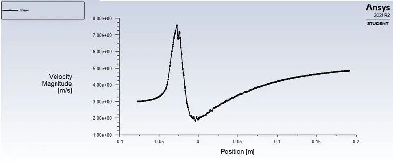
Velocity vs Length Plot
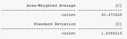
- Compare with the Analytical Temperature calculated from the formula is `T_(mixture)=30.32209^oC`.
CASE 4 (MOMENTUM RATIO 4) FOR LONG MIXING TEE
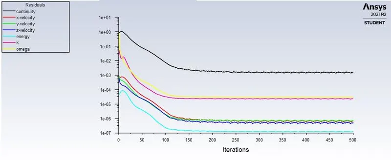
- The solution is converged at 500 iterations
The residual for the governing and transport Equation is given by
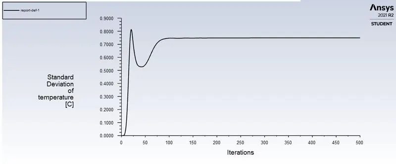
Standard Deviation of the Temperature of outlet is given by
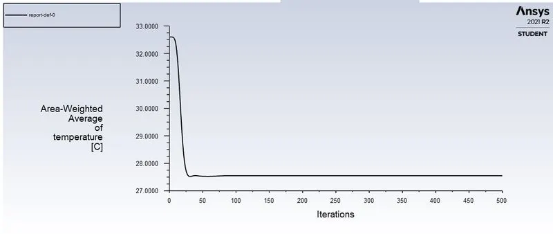
Area Weighted Average of Temperature Outlet
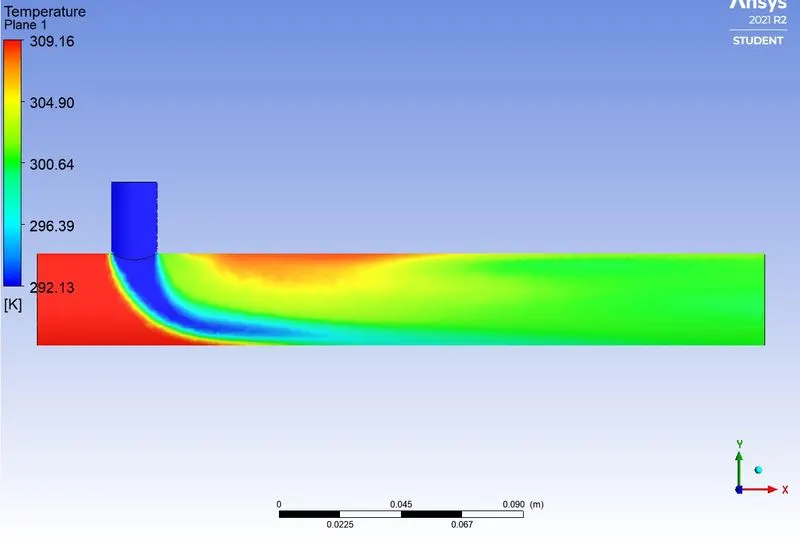
Temperature plot is given by
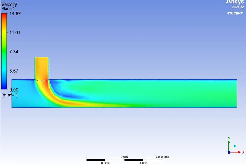
Velocity Plot is given by
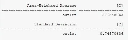
- Compare with the Analytical Temperature calculated from the formula is `T_(mixture)=27.4872^0C`
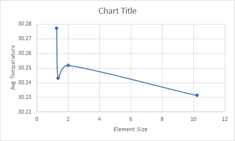
Mesh Independent test:(Mixing Test short Momentanum Ratio 2 )
| Size (mm) | Elements | Temperature(Degree celcius) |
| 10.219 | 12441 | 30.2314 |
| 1.25 | 329296 | 30.277374 |
| 1.35 | 271136 | 30.24315 |
| 2 | 104950 | 30.25186 |
Conclusion:
- The Momentum Ratio i.e., The Inlet velocity of the cold and hot influence the Average Outlet Temperature.
- Increase on the Momentum Ratio the average outlet temperature decreases.
- From the above case, the length has a small or negligible effect on the Average outlet temperature.