Week 1- Mixing Tee
MIXING TEE CFD SIMULATIONS
ABSTRACT
This project is about Computational Fluid Dynamics-based mixing effectiveness analysis of a short and long mixing tee for different momentum ratios. Steady-state simulations were performed for mixing tee in two cases. The first case is a short mixing tee with a hot fluid inlet velocity of 3 m/s and momentum ratios 2 and 4. The second case is a long mixing tee with a hot fluid velocity of 3 m/s and momentum ratios 2 and 4. Two turbulent models (k-epsilon and k-omega) are applied to the first and the k-epsilon model is applied to the second case. The mixing effectiveness was observed using ANSYS FLUENT software.
FORMULA
Momentum ratio=inlet velocity of hot fluid/inlet velocity of cold fluid.
OBJECTIVES
- To generate temperature and velocity contour and line plots of fluid.
- To perform Mesh independent study on one case.
- To compare 1.Cell count 2.Average outlet temperature 3.No.of iterations for convergence for each case.
- To compare Analytical solutions with numerical solutions obtained by simulations.
INTRODUCTION
In industries, mixing tee is widely used for mixing the different fluids of different temperatures to get desired output temperatures, and also it is used to convert the Heterogeneous system to more Homogeneous. Mixing tee utilizes a specifically engineered internal geometry to efficiently mix two fluid streams into one combined homogeneous stream.
The applications of mixing tees are in the petrochemical, HVAC, electronic industries, and nuclear power plants. Computational fluid dynamics uses Mathematics, Physics, and computational software to visualize how fluid flows and affects it's medium and neighbors. ANSYS FLUENT is the software that predicts flow phenomena based on some governing equations like conservation of energy and conservation of momentum.
TURBULENT MODELS
In this problem, two models namely k-epsilon and k-omega are used. K-epsilon is the widely used common model in CFD to simulate mean flow characteristics for turbulent flow conditions. It is a two-equation model that uses two transport equations (PDEs).
- The first transported variable is the turbulent kinetic energy (k).
- The second transported variable is the rate of dissipation of turbulent kinetic energy (ε).
K-epsilon model is well suited for predicting the solutions in areas that are far from the walls.
The k–omega turbulence model is also a common two-equation turbulence model, that is used as an approximation for the Reynolds-averaged Navier-Stokes equation (RANS equations). The model attempts to predict turbulence by two partial differential equations for two variables, k and ω, with the first variable being the turbulent kinetic energy (k) while the second (ω) is the specific rate of dissipation (of the turbulence kinetic energy k into internal thermal energy).
k-omega model is well suited for the simulations to flow in viscous sub-layer.
FLOW CHART FOR SOLVING AND MODELLING APPROACH
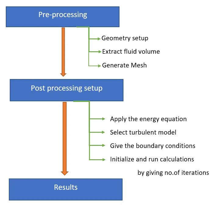
PRE-PROCESSING :
GEOMETRY
- Open the ANSYS SpaceClaim geometry from the Ansys workbench and import the mixing tee geometry.
- Extract the fluid volume and suppress the shell to view fluid volume.
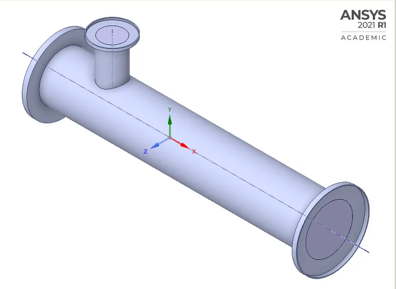
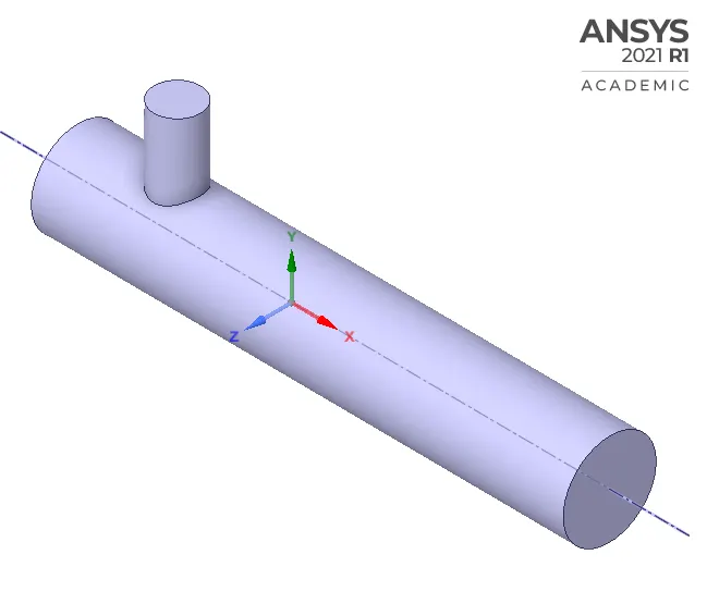
Fig.Mixed tee Fig.Extracted fluid volume
- Now close the SpaceClaim and open the Mesh
MESHING
- Suppress the shell to view the fluid volume and name the sections as inlet x, inlet y, outlet, and wall with the help of create named selection option.
- Click on Generate mesh for meshing.
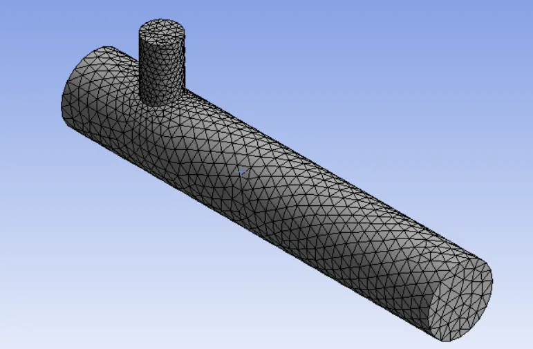
- To view the mesh quality click on the mesh matrics.
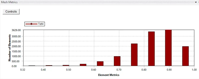
- From the table, we can say that the more no. of elements are above 60 to 70% quality. so the mesh is acceptable.
FLUENT SETUP
- Solver type: Pressure-Based
- Velocity formulation: Absolute
- Type: Steady
- Model: Realizable k-epsilon/k-omega SST
- Material: fluid as Air
- Boundary conditions: inlet x, velocity=3m/s, temperature=36°C inlet y, velocity=6m/s for momentum ratio=2 velocity=12m/s for momentum ratio=4, temperature=19°C
- Initialization: Hybrid initialization.
SOLUTIONS
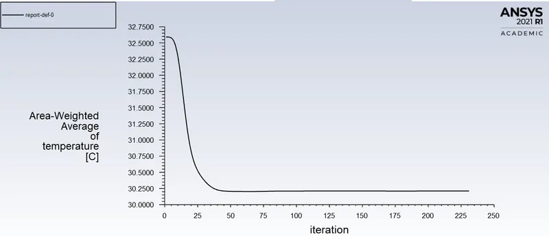
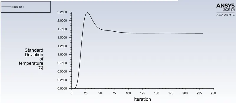
- Creat the area-weighted temperature and standard deviation of temperature at outlet using definitions option
- Now run the calculations by giving no. of iterations
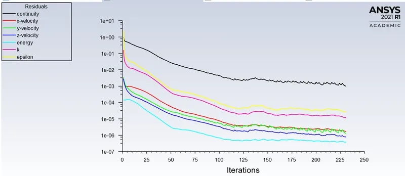
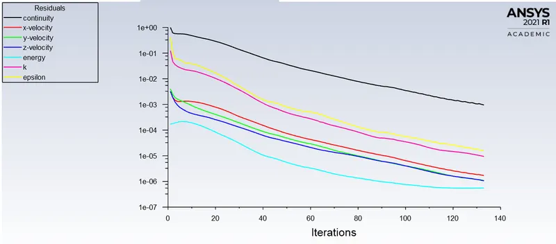
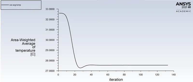
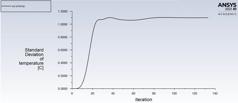
- After some time the solutions will be converged. So that we can visualize the Residuals, Area-weighted average temperature, and standard deviation of temperature.
POST-PROCESSING RESULTS:
CASE 1)SHORT TEE
MODEL: k-epsilon
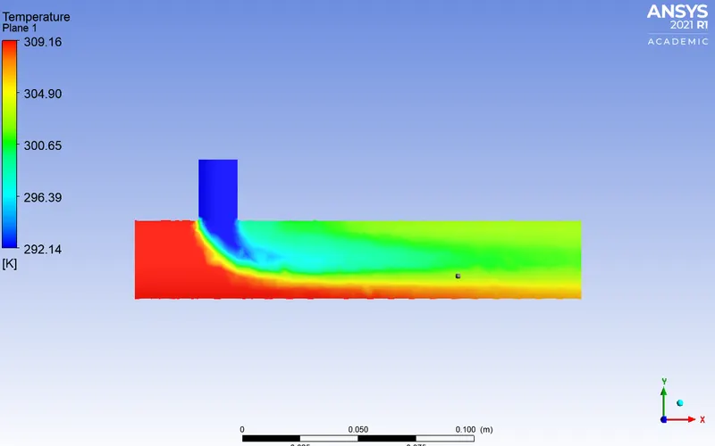
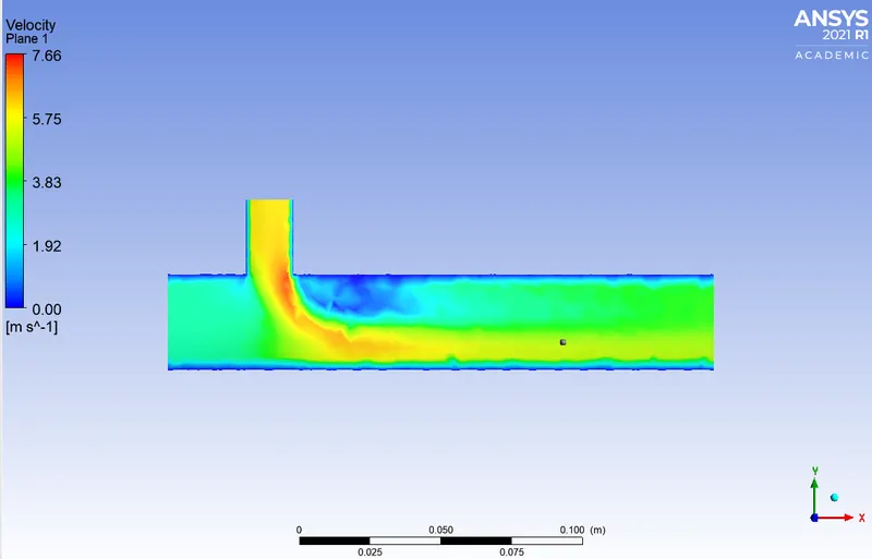
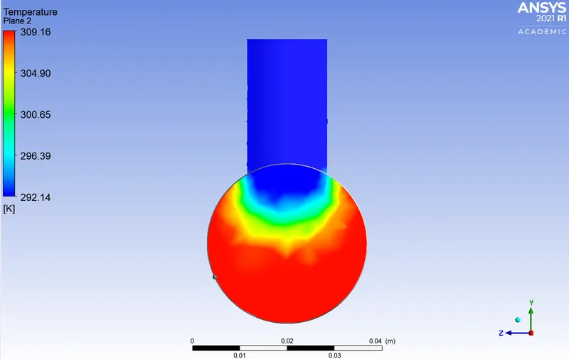
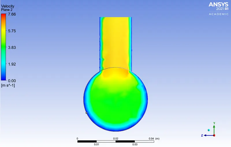
MOMENTUM RATIO=2
CONVERGENCE PLOTS
Residuals
Area-weighted average temperature
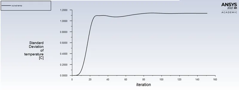
Standard deviation of temperature
CONTOUR PLOTS
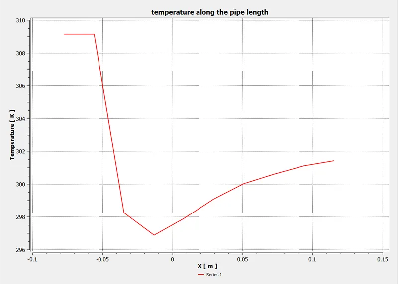
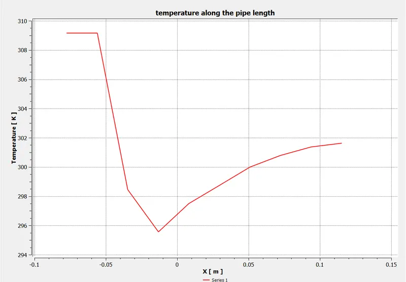
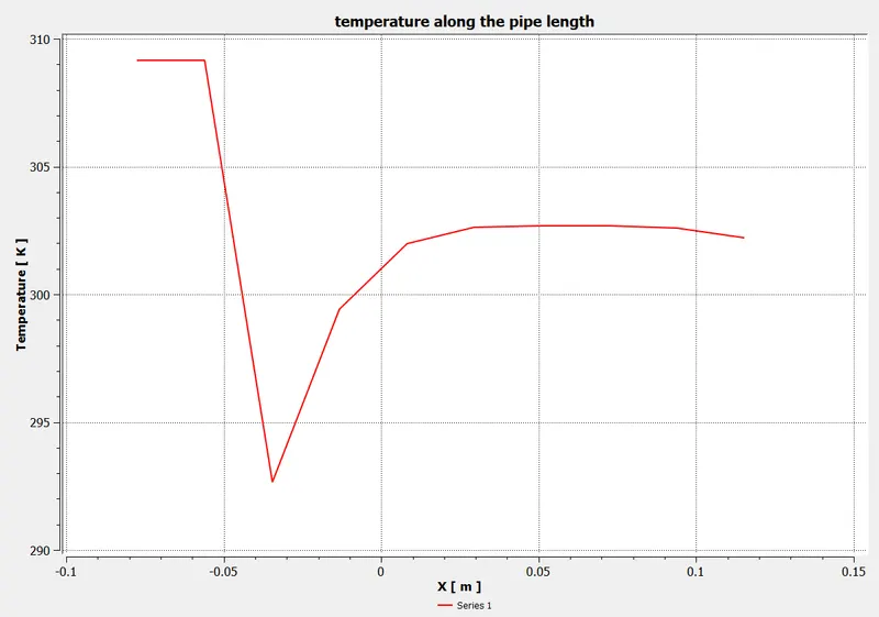
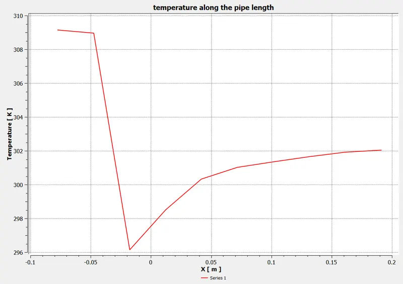
Temperature along the pipe length
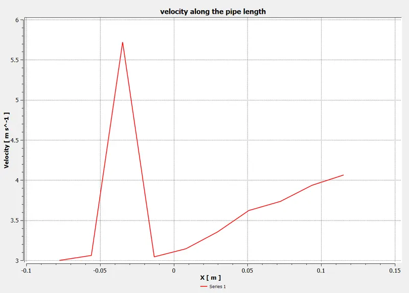
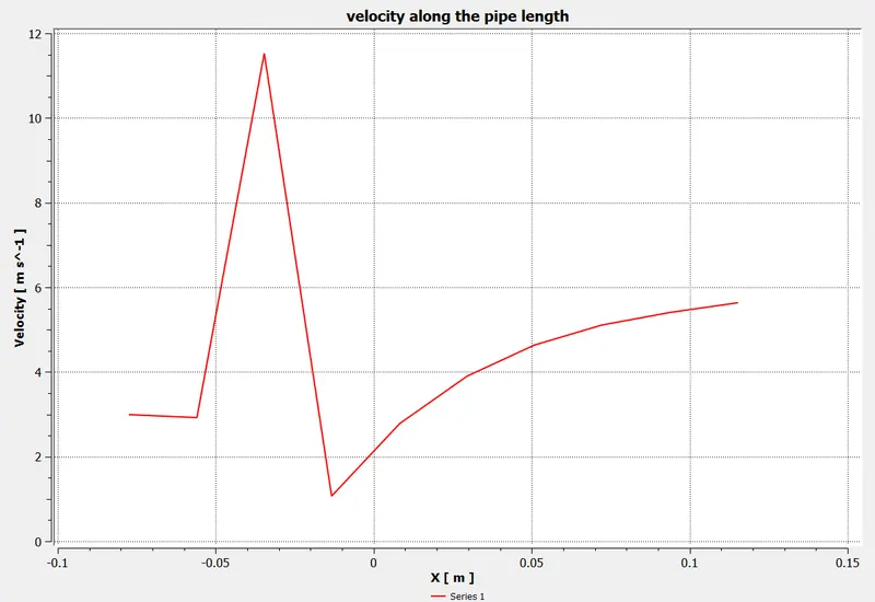
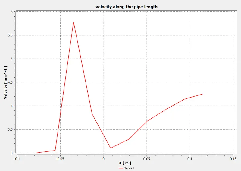
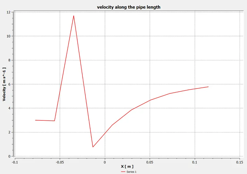
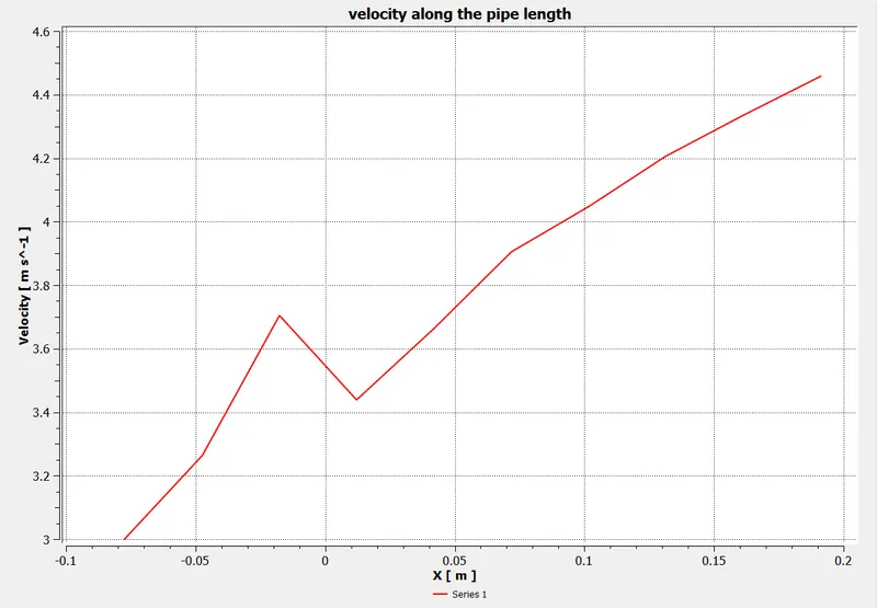
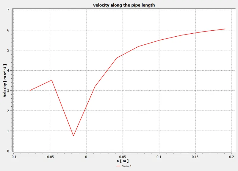
Velocity along the pipe length
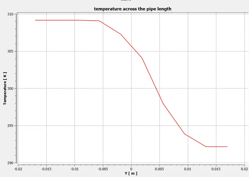
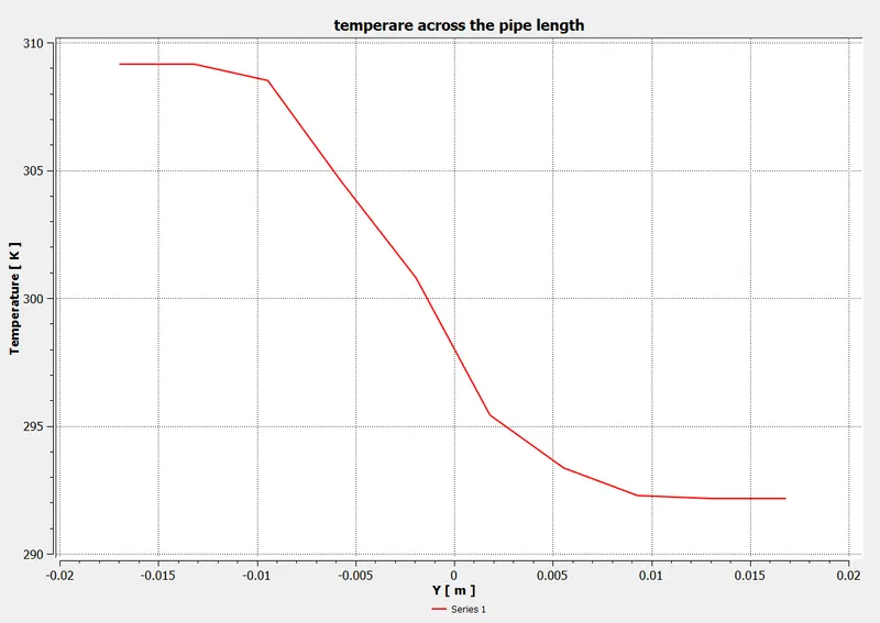
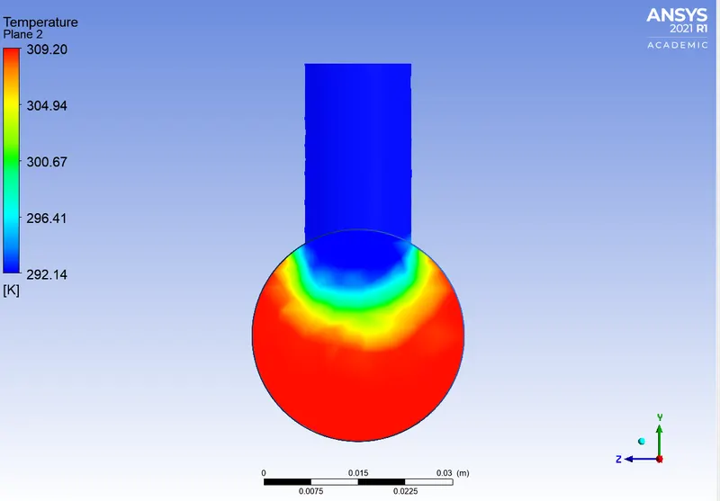
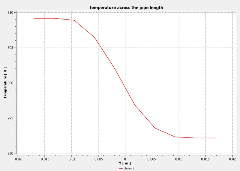
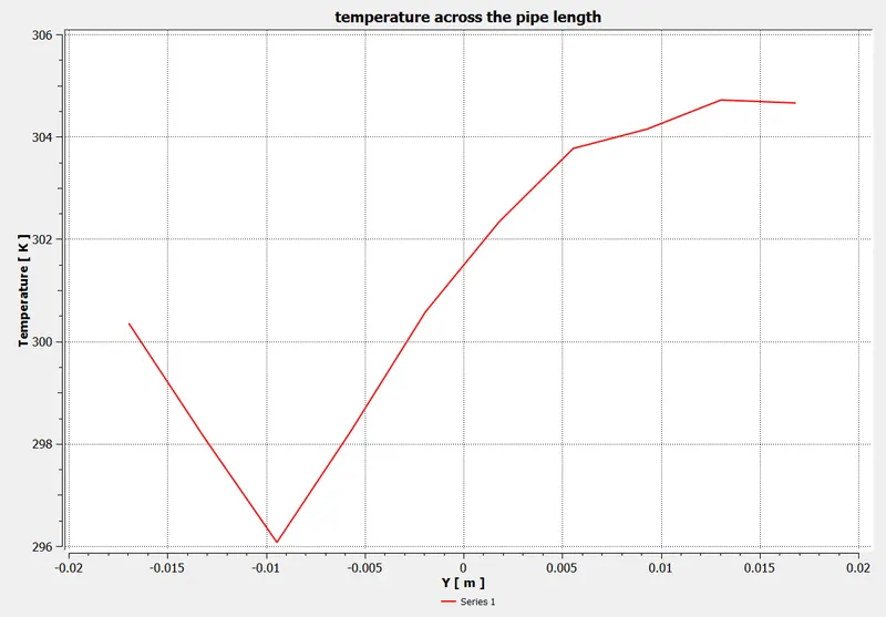
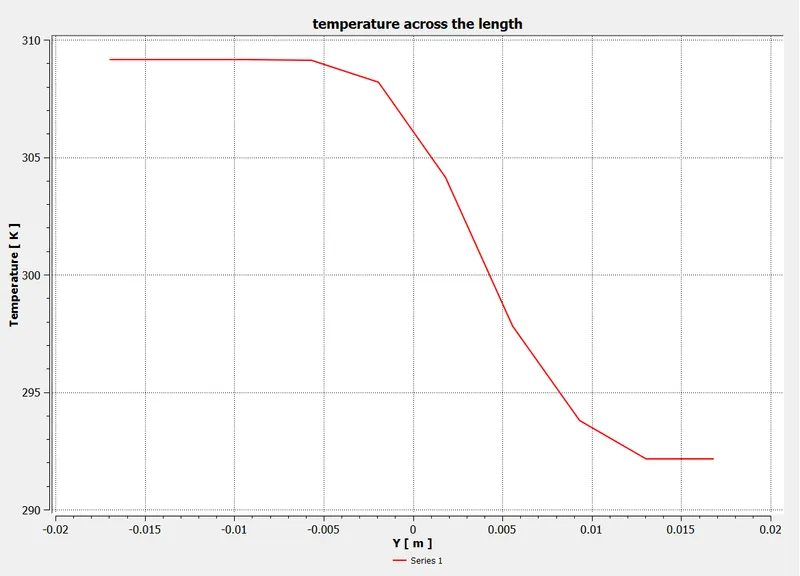
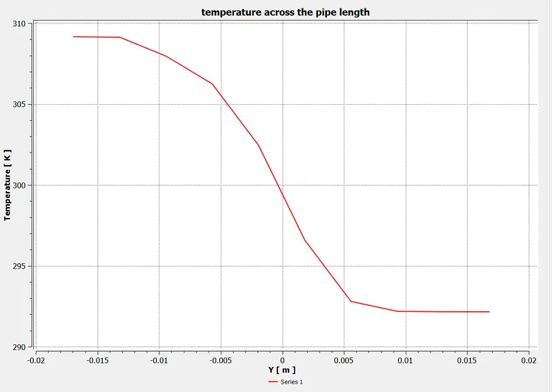
Temperature across the pipe length
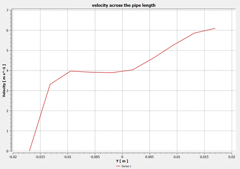
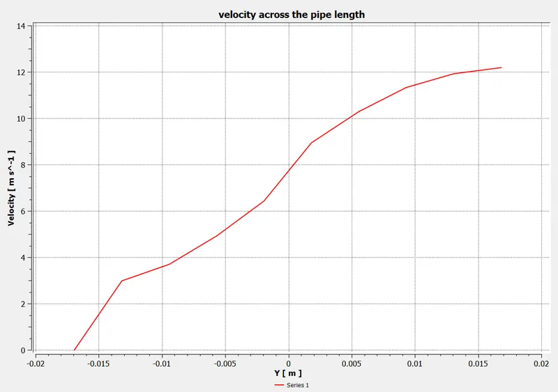
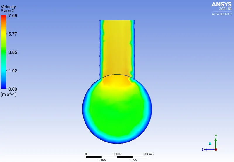
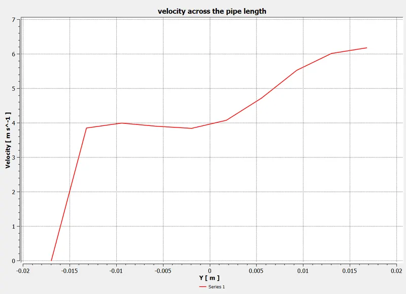
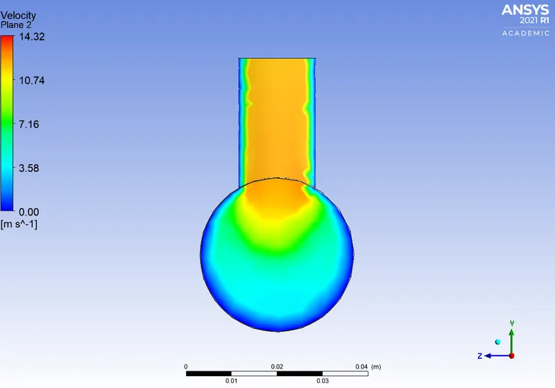
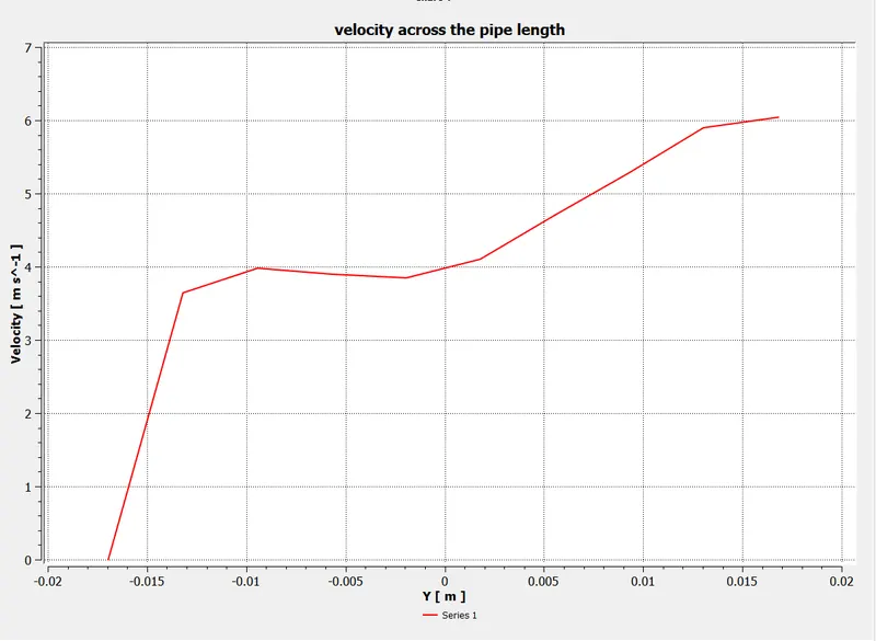
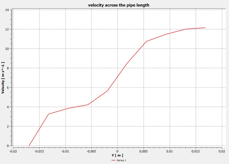
Velocity across the pipe length
LINE PLOTS:
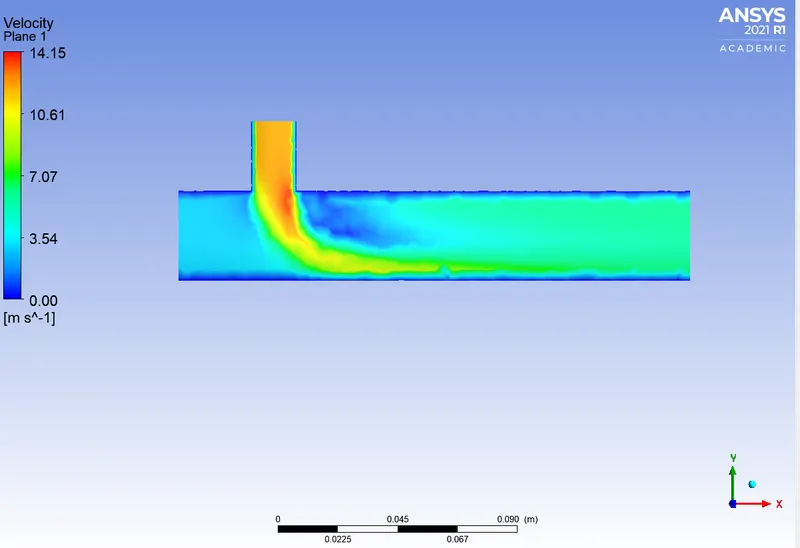
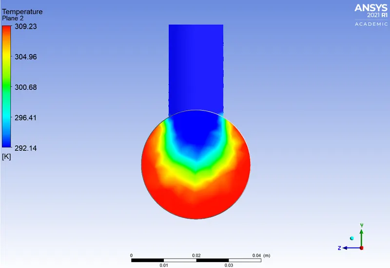
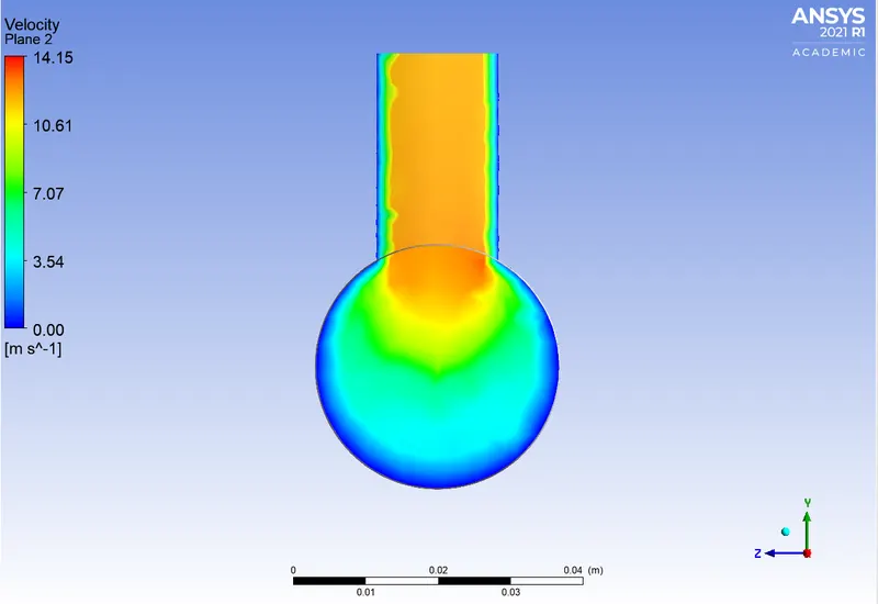
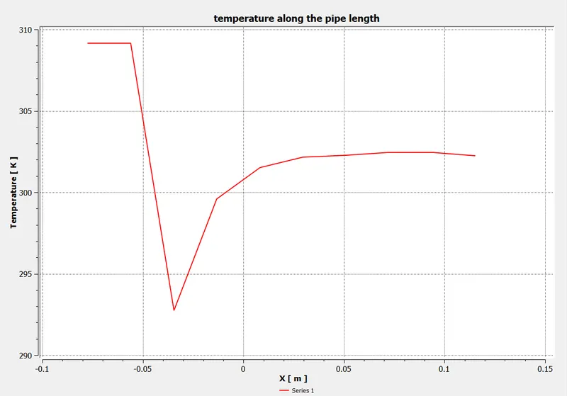
MOMENTUM RATIO=4
CONVERGENCE PLOTS
Residuals
Area-weighted average temperature
Standard deviation of temperature
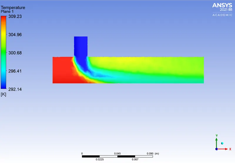
CONTOUR PLOTS
Temperature along the pipe length
Velocity along the pipe length
Temperature across the pipe length
Velocity across the pipe length
LINE PLOTS:
MODEL: k-omega
MOMENTUM RATIO=2
CONVERGENCE PLOTS
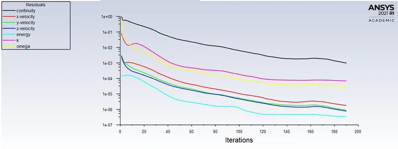
Residuals
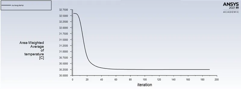
Area-weighted average temperature
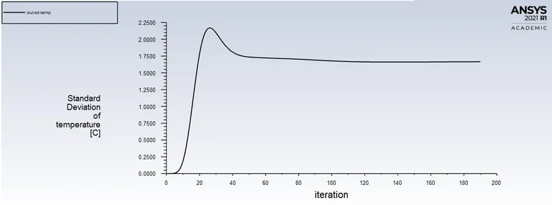
Standard deviation of temperature
CONTOUR PLOTS
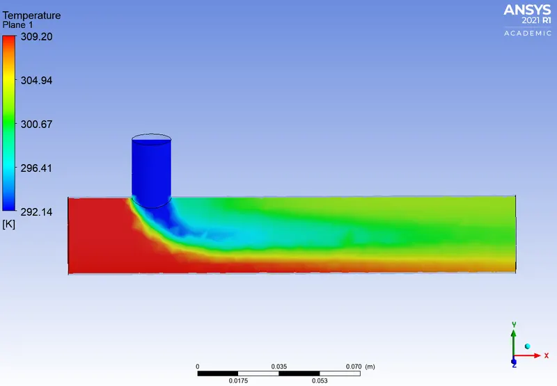
Temperature along the pipe length
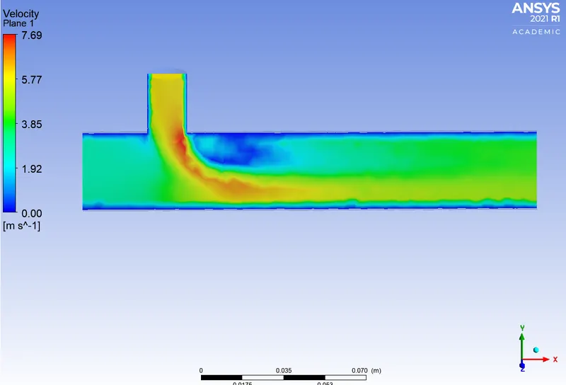
Velocity along the pipe length
Temperature across the pipe length
Velocity across the pipe length
LINE PLOTS:
MOMENTUM RATIO=4
CONVERGENCE PLOTS
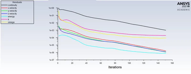
Residuals
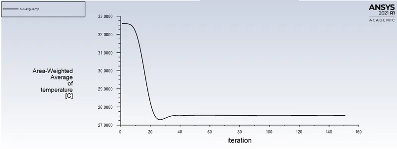
Area-weighted average temperature
Standard deviation of temperature
CONTOUR PLOTS
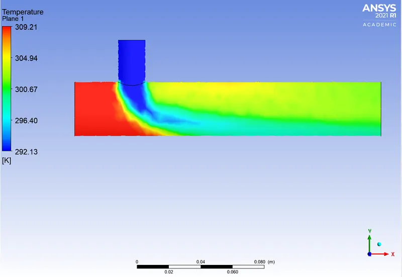
Temperature along the pipe length
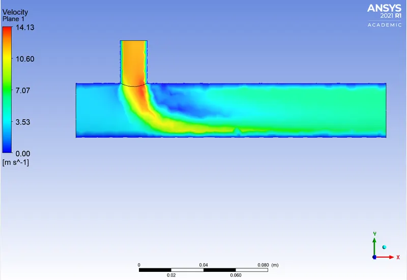
Velocity along the pipe length
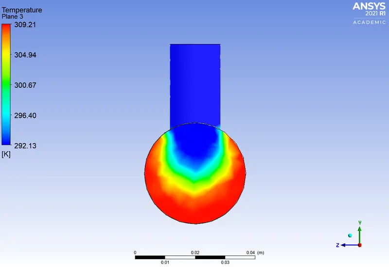
Temperature across the pipe length
Velocity across the pipe length
LINE PLOTS:
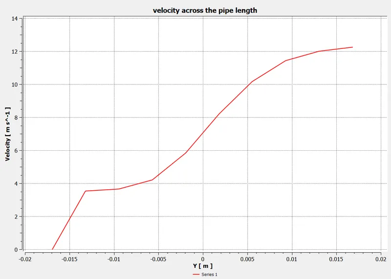
CASE 2) LONG TEE
MODEL: k-epsilon
MOMENTUM RATIO=2
CONVERGENCE PLOTS
Residuals
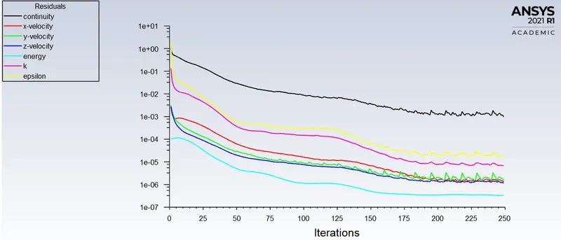
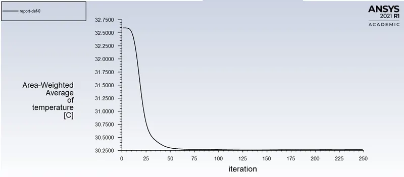
Area-weighted average temperature
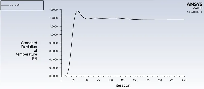
Standard deviation of temperature
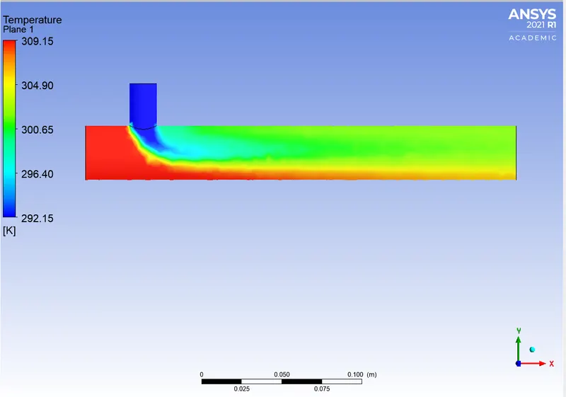
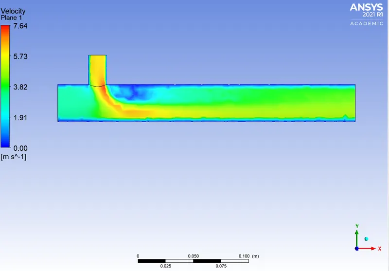
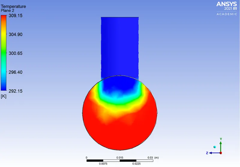
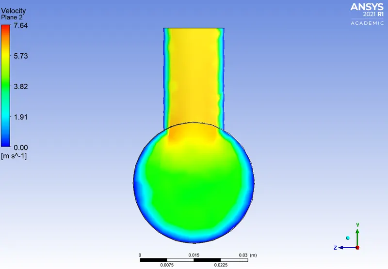
CONTOUR PLOTS
Temperature along the pipe length
Velocity along the pipe length
Temperature across the pipe length
Velocity across the pipe length
LINE PLOTS:
MOMENTUM RATIO=4
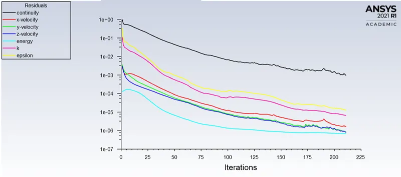
CONVERGENCE PLOTS
Residuals
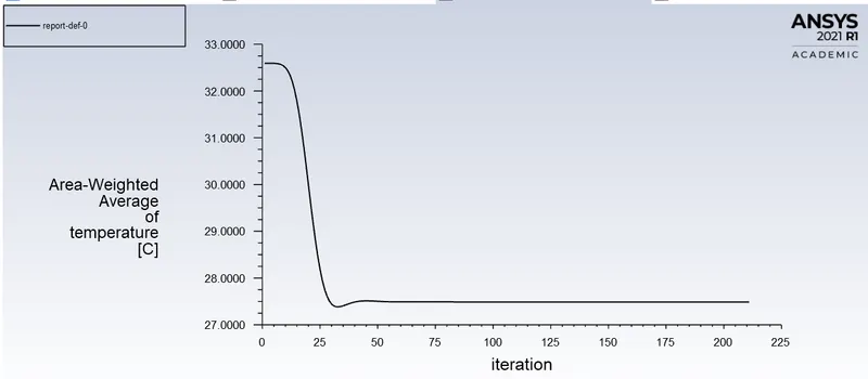
Area-weighted average temperature
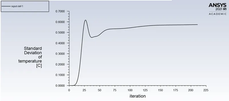
Standard deviation of temperature
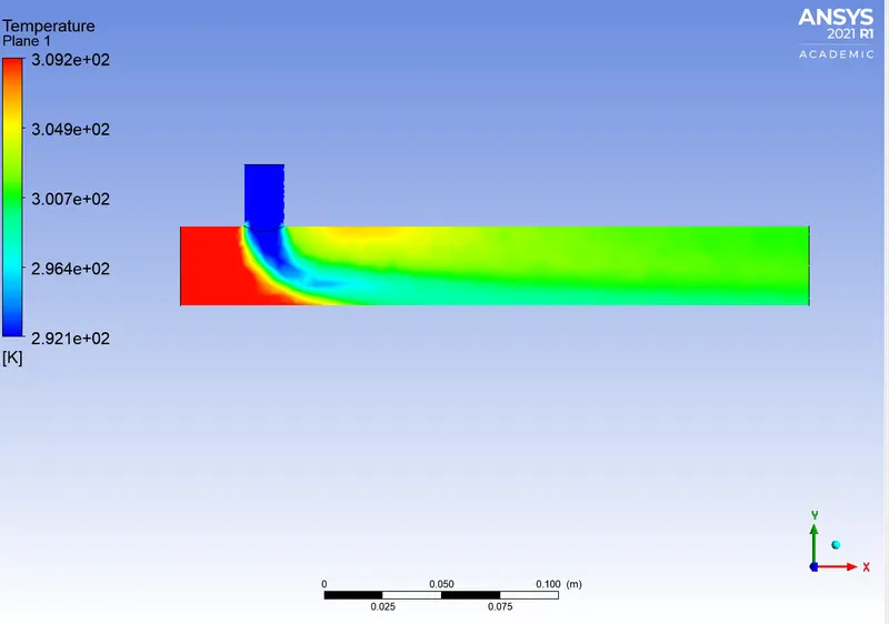
CONTOUR PLOTS
Temperature along the pipe length
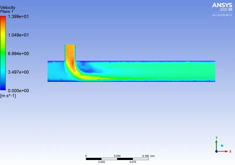
Velocity along the pipe length
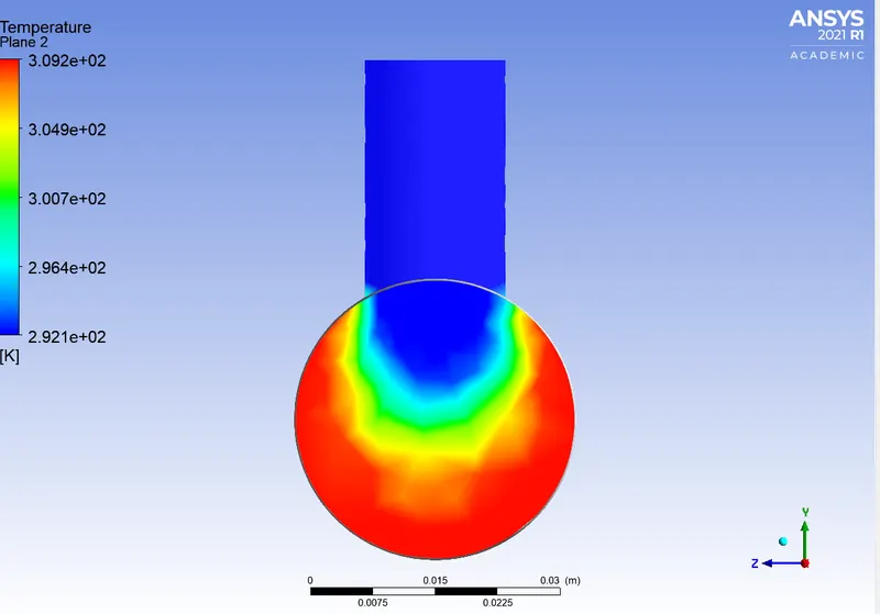
Temperature across the pipe length
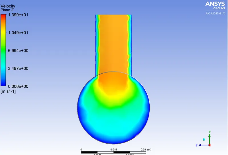
Velocity across the pipe length
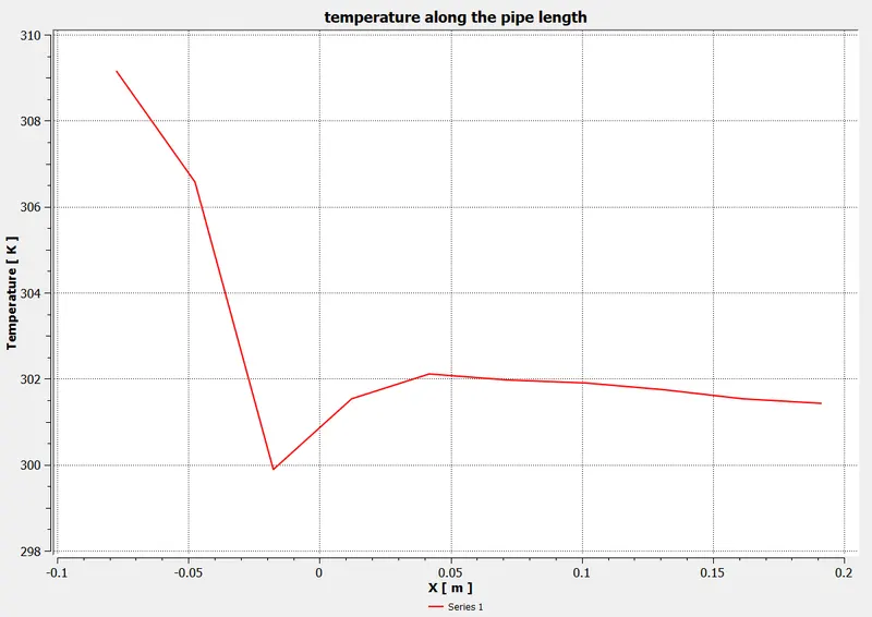
LINE PLOTS:
NUMERICAL SOLUTIONS - RESULTS
MODEL: k-epsilon
| Geometry | Momentum Ratio | Cell count | Average outlet temperature (°C) | no. of iterations for convergence |
| Short tree | 2 | 14330 | 30.21 | 231 |
| Short tree | 4 | 12760 | 27.54 | 133 |
| Long tee | 2 | 15689 | 30.26 | 249 |
| Long tee | 4 | 15689 | 27.48 | 211 |
MODEL: k-omega
| Geometry | Momentum Ratio | Cell count | Average outlet temperature (°C) | no. of iterations for convergence |
| Short tee | 2 | 12657 | 30.25 | 228 |
| Short tee | 4 | 12657 | 27.51 | 131 |
ANALYTICAL SOLUTIONS:
SHORT TEE
MOMENTUM RATIO=2
Known inputs are
Dx=33.876mm, Dy=16.962mm
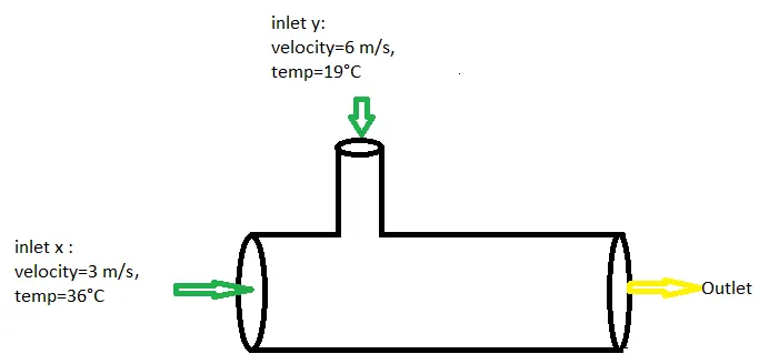
Fig.Mixing tee
apply conservation of energy
(mh)x+(mh)y=(mh)out.....(1)
m=ρAV, h=cT, Assume density and specific heats are constant.
(m)x+(m)y =(m)out
(ρAV)x+(ρAV)y=(ρAV)out
by substituting all the values, Vout=4.504m/s
from (1), (ρAVcT)x+(ρAVcT)y=(ρAVcT)out
by substituting all the values, Tout=30.324°C
MOMENTUM RATIO=4
Here, the only one change is inlet y velocity =12 m/s
by following the same procedure and substituting all the values
Vout=6.0086m/s, Tout=27.487°C
LONG TEE
MOMENTUM RATIO=2
Known inputs are Dx=34.876mm, Dy=16.9625mm
Vx=3m/s, Vy=6m/s.
by following the same procedure and substituting all the values
Vout=4.4193m/s, Tout=30.5402°C
MOMENTUM RATIO=4
Here, the only one change is inlet y velocity =12 m/s
by following the same procedure and substituting all the values
Vout=5.8386m/s, Tout=27.735°C
COMPARISON OF ANALYTICAL AND NUMERICAL SOLUTIONS
| Geometry | Momentum ratio |
ANALYTICAL RESULTS Average temperature at the outlet (°C) |
NUMERICAL RESULTS Average temperature at the outlet (°C) k-epsilon model |
NUMERICAL RESULTS Average temperature at the outlet (°C) k-omega model |
| Short tee | 2 | 30.32 | 30.21 | 30.25 |
| Short tee | 4 | 27.48 | 27.54 | 27.51 |
| Long tee | 2 | 30.54 | 30.26 | |
| Long tee | 4 | 27.73 | 27.48 |
MESH INDEPENDENT STUDY FOR SHORT TEE (MR=2, k-epsilon model)
|
Mesh size(mm) |
No. of elements | No. of nodes | No. of iterations | Avg outlet temperature(°C) |
| 5 | 14202 | 3127 | 167 | 30.28 |
| 3 | 39803 | 8343 | 120 | 30.205 |
| 1.1 | 454823 | 87800 | 126 | 30.406 |
CONCLUSIONS
- On comparing analytical and numerical solutions, we can say that both the solutions are almost equal. k-omega and k-epsilon, both models giving nearer values when compared with analytical solutions.
- Based on Mesh independent study, we can say that the mesh size of 3mm giving almost the nearest value. But remaining all the results are also nearer values. so our model is independent of the mesh size.
- Long tee is suitable for better mixing of fluids and gives the best predictions for the solutions.
- The high value of momentum ratio gives better mixing efficiency and by that, it gives a homogeneous stream at the outlet.
- From the results, we can conclude that created model is well suited for the present problem.