Week 1: Channel flow simulation using CONVERGE CFD
Channel Flow Simulation using Converge CFD
Introduction: Flow through channel is a common phenomenon observed in many engineering applications. The physics of flow in a channel or a closed boundary can be best described by the forces governing the cause of flow i.e., energy gradient and friction encountered at the boundary layer. A steady flow in a rectangular channel is often characterized by zero velocity at the boundary layer and maximum velocity at the core.
The scope of present study is to achieve the steady flow using a proprietary tool for computational tool fluid dynamics (CFD) CONVERGE CFD v3.016
Aim: To develop a computational model for flow of gas through rectangular channel and to study the impact of 3 different mesh sizes on the flow.
Outline: The objective of the study has been carried out in following three cases.
Case 1: Grid Size of 2e-4 m
Case 2: Grid Size of 1.5e-4 m
Case 3: Grid Size of 1e-4 m
Geometry Definition:
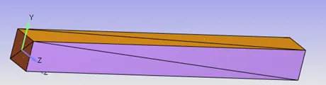
Using the geometry module in converge, a box type geometry is made centered at (0.05, 0, 0) and length in x direction of 0.1 m also, with width and height in y and z- axis of 0.01m.
Boundary Names:
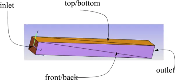
The image with boundary names has been provided below.
Boundary Definition:
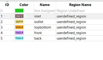
As per boundary names the following boundary were defined
Inlet:
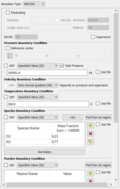
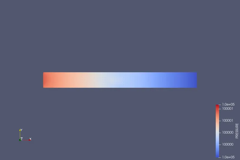
The inlet is of inflow boundary condition with specified pressure of 100001Pa.
Outlet:
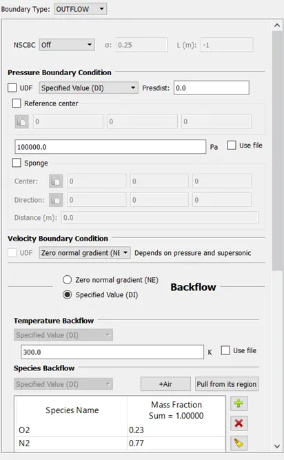
The outlet is specified as outflow boundary condition with a pressure of 100000Pa.
Top and Bottom:
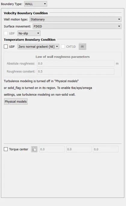
Top and bottom is given the wall boundary condition of no slip.
Front and Back:
Front and back is given 2d boundary condition

Definition of Regions:
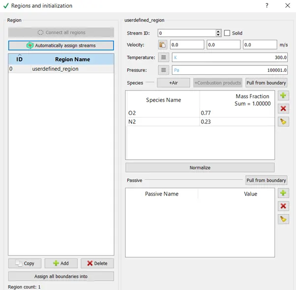
The new region is named as userdefined_region. Here, the initial pressure condition is set as 100001Pa, same as that of inlet. The region is prescribed for the boundaries.
Materials
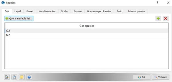
Air has been chosen as the gas flowing through rectangular channel.
Case Setup
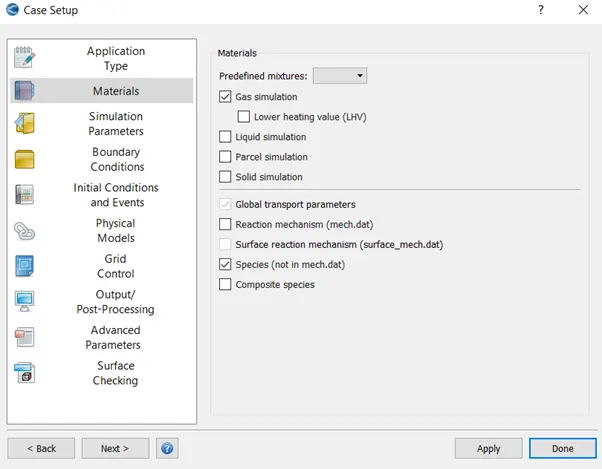
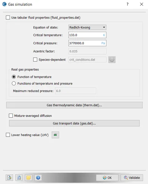
Gas Simulation
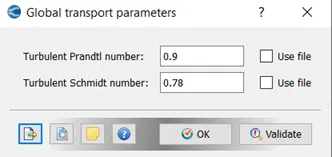
Global Transport Parameters
Species
Simulation Parameters
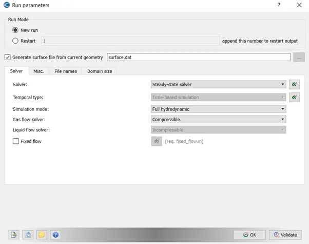
Run Parameters
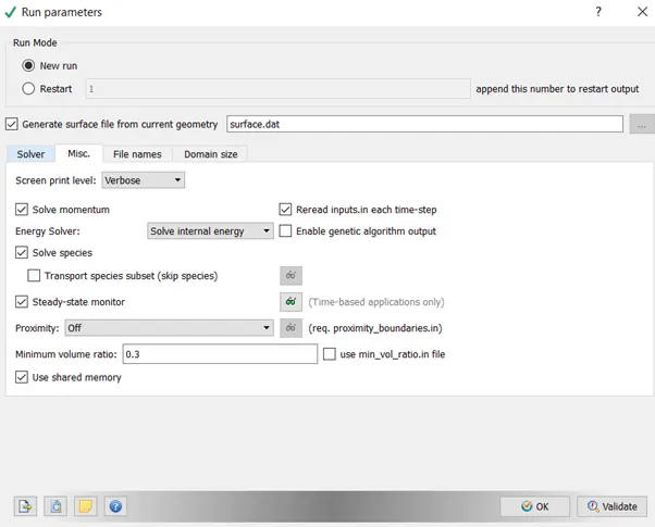
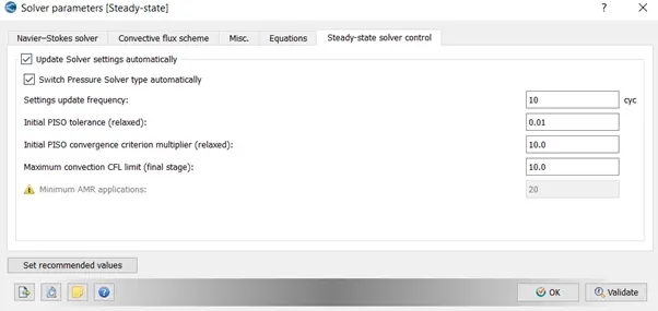
Steady State Solver with full hydrodynamic simulation mode has been used. The gas flow in the simulation is assumed to be compressible.
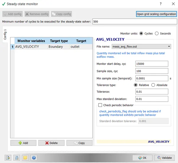
Steady State monitor has been turned on.
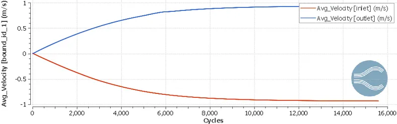
Average velocity at the out let is the monitored variable, with first check for converge set at 15000 cycles.
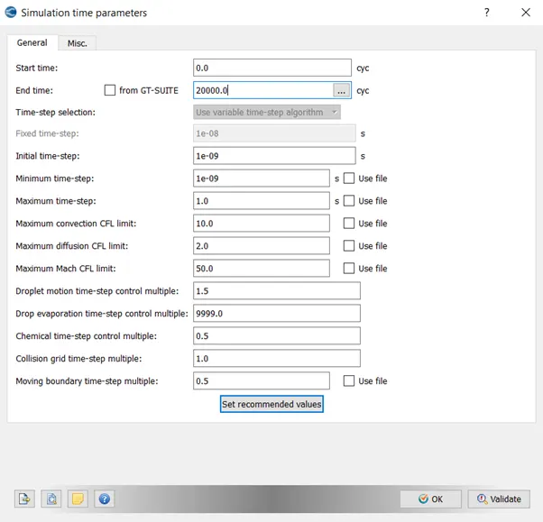
Simulation time parameter
20000 cycles have been used as the maximum no. of cycles with a minimum and maximum time step size of 1e-9s.
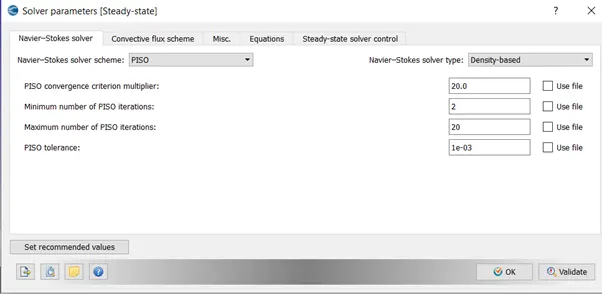
Solver Parameter
Density based solver has been used.
Physical Models
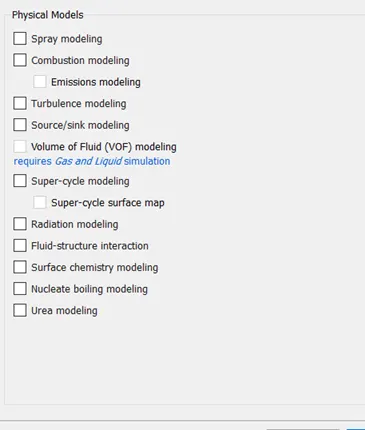
No turbulence model is being used.
Grid Size
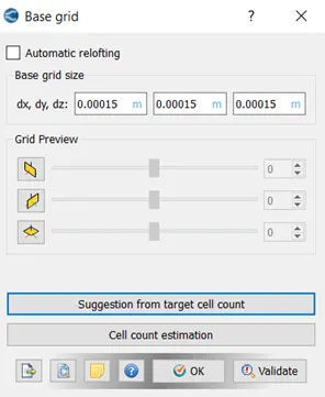
As described above, the grid size is varied in three steps, 2e-4m, 1.5e-4 and 1e-4m.
Output Variables/Files
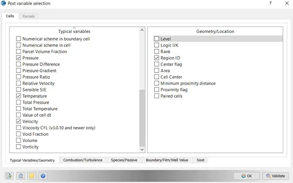
Density pressure temperature and Velocity variables is chosen as the post variable selection.
Output files
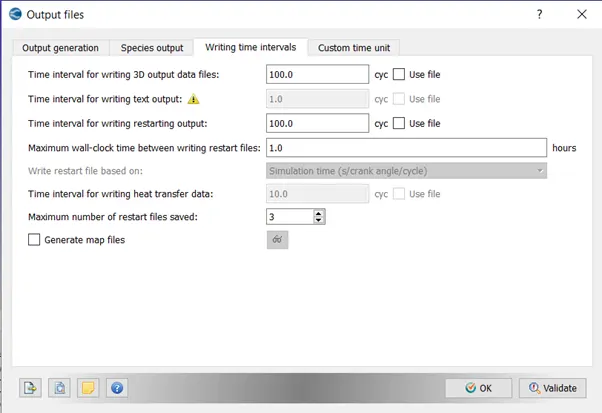
Results:
Case 1:
Animation:
Grid View:

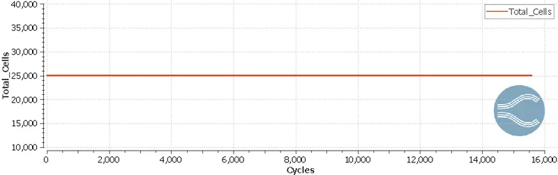
Cell Count:
Contour Plot:
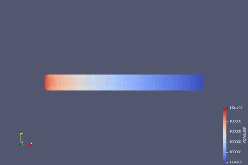
Pressure
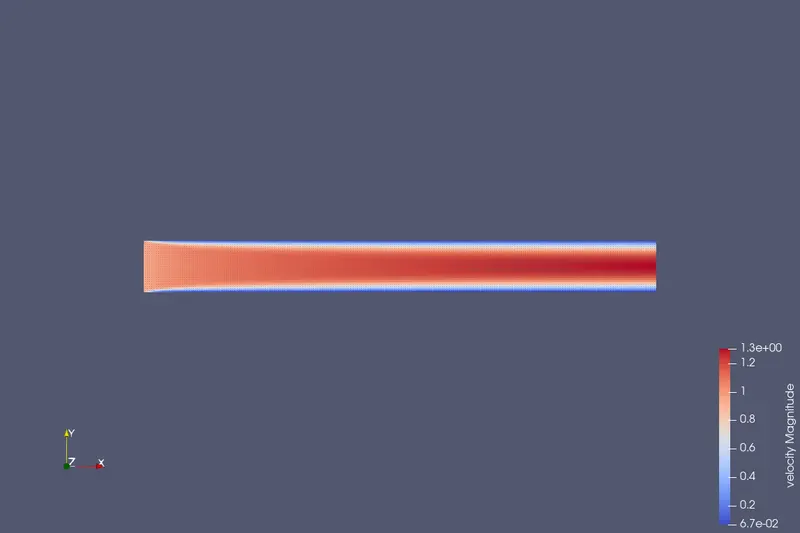
Velocity
Line Plot Cross-Section:
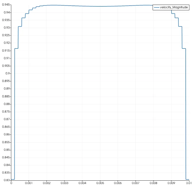
Velocity at inlet:
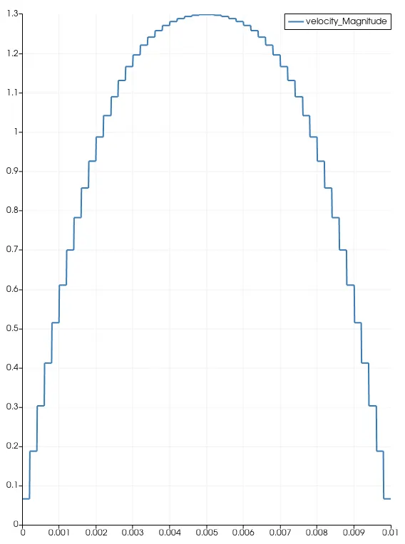
Velocity at outlet:
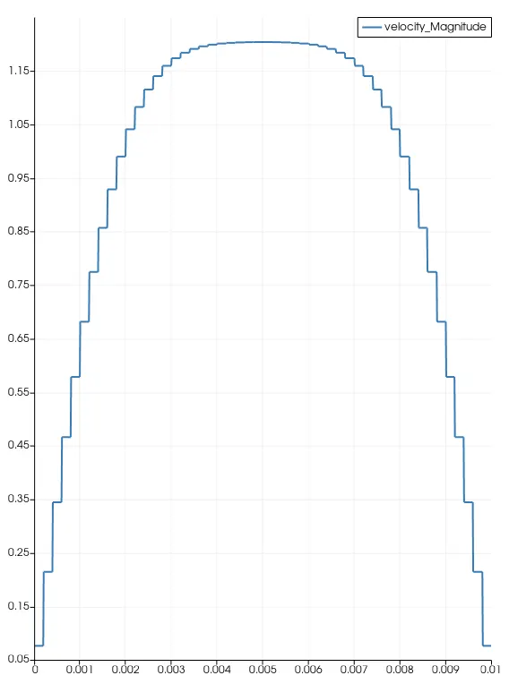
Velocity at mid:
Boundary Plot:
Average Velocity:
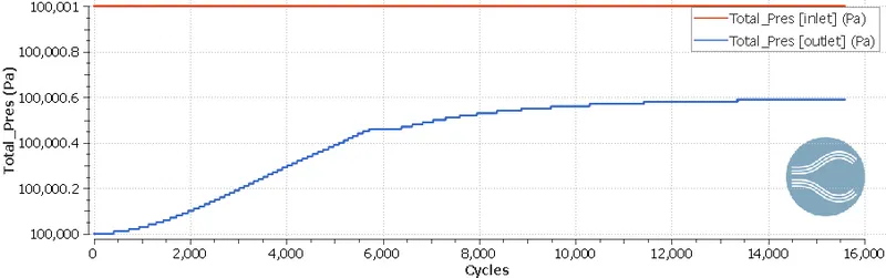
Total Pressure:
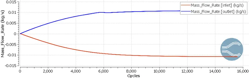
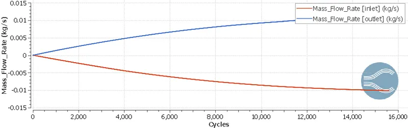
Mass Flow Rate:
Case 2:
Animation:
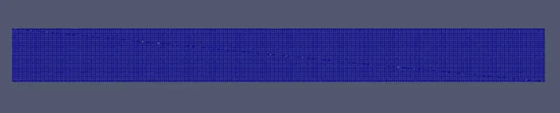
Grid View:
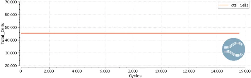
Cell Count:
Contour Plot:
Pressure
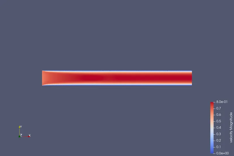
Velocity
Line Plot Cross-Section:
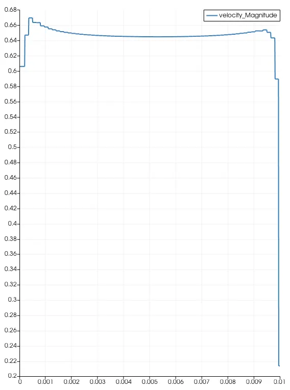
Velocity at inlet:
Velocity at outlet:
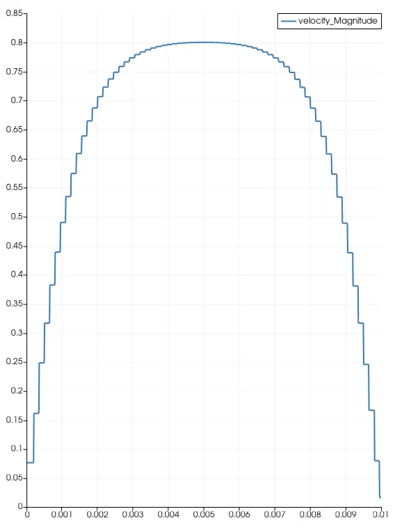
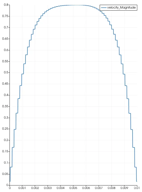
Velocity at mid:
Boundary Plot:
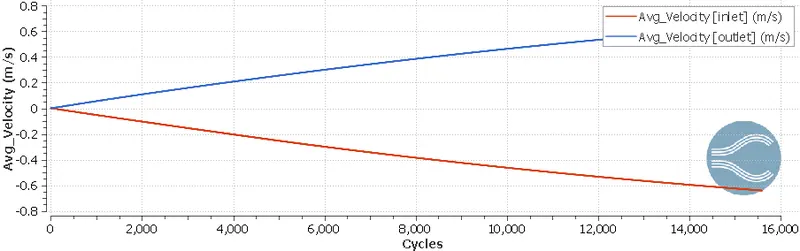
Average Velocity:
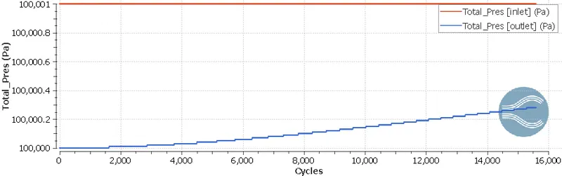
Total Pressure:
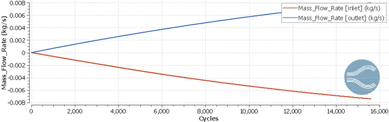
Mass Flow Rate:
Case 3:
Animation:
Grid View:

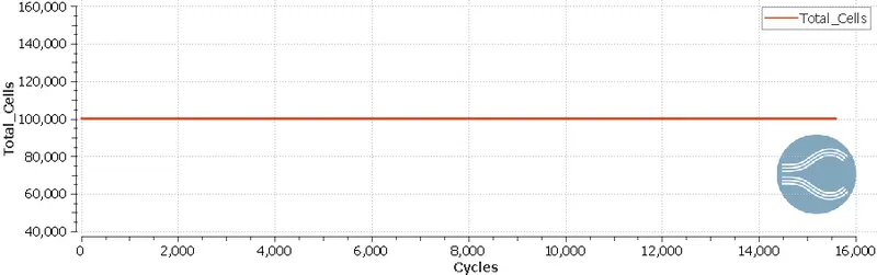
Cell Count:
Contour Plot:
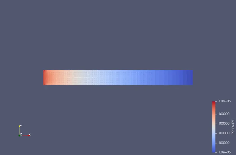
Pressure
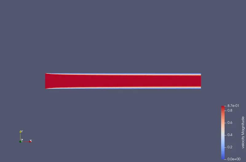
Velocity
Line Plot Cross-Section:
Velocity at inlet:
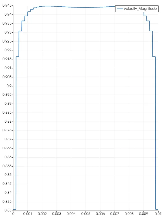
Velocity at outlet:
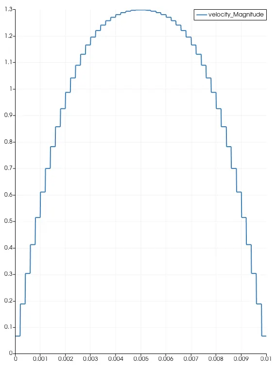
Velocity at mid:
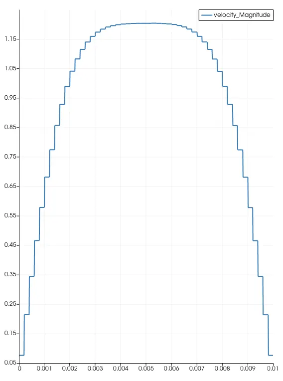
Boundary Plot:
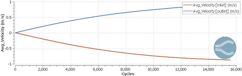
Average Velocity:
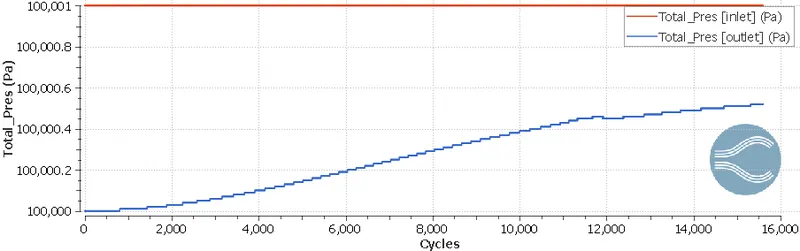
Total Pressure:
Mass Flow Rate:
Conclusions:
1. As we decrease the grid size, the no. of cell count increases. The cell count remains constant throught the simulation for a particular grid size as there is no dynamic mesh generation.
2. In the plots with respect to no. of cycles, after a few cycle the change in values of variables began to slow down. After certain iterations, the convergence is reached and we are presented with appropriate values.
3. Steady flow inside the channel is developed wchi can be seen by the cross-section plots at 3 different lengths. At inlet, the curve appears to be rectangular with a fairly flat line in the pipe. At the outlet, a steady parabolic velocity curve is found.
4. Pressure at inlet remains same whereas, the pressure at outlet raises up slightly to reach that of inlet.
5. For a highest grid size the maximum velocity is over approximated as compared with the lower grid sizes.